This chapter presents new indicators on the economy of African cities that are based on data from more than 4 million individuals from across Africa. The indicators provide a new perspective on African cities that is unprecedented in its breadth and level of detail. They make it possible to compare the performances of cities of different sizes, document the corresponding evolution over time and analyse the effects of cities on nearby rural areas. The results show the positive impact that urbanisation has on economic performance and quality of life in almost all measurable dimensions.
Africa’s Urbanisation Dynamics 2022

1. New evidence on Africa’s urban economy
Abstract
In Brief
The policy debate on urbanisation in Africa has long suffered from a paucity of reliable data. This chapter presents new evidence on African cities based on data from more than 4 million individuals across 2 600 cities in 34 countries, working both in the formal and in the informal economy. Matching individuals to cities based on the co-ordinates of their place of residence makes it possible to describe African cities at an unprecedented level of detail.
The data shows that urbanisation in Africa has contributed substantially to better economic outcomes and living standards. Within their countries, African cities outperform in most dimensions. Hourly wages in large cities are twice as high as in rural areas, and underemployment is less prevalent, since urban workers work 30% more hours per week than rural workers. The share of workers in skilled occupations is approximately 50% among men and 25% among women in midsized and large cities, but only 18% and 11%, respectively, in rural areas.
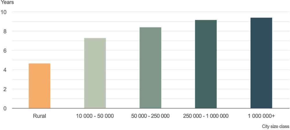
One of the key advantages of cities is that they facilitate access to services and infrastructure. Children in large cities receive almost five years more education on average than children in rural areas. In large cities, 80% of households are connected to the electricity grid, but only 20% of households in rural areas are. More than half of all households in large cities have a bank account, whereas the share in rural areas is less than 20%.
Figure 1.1. Average years of schooling of residents aged 18-29 by city size
Note: Based on Demographic and Health Surveys from various years between 2010-19 for AGO, BEN, BFA, BDI, CIV, CMR, COD, COM, GAB, GHA, GIN, KEN, LBR, LSO, MDG, MLI, MOZ, MWI, NAM, NGA, RWA, SEN, SLE, TCD, TGO, TZA, UGA, ZAF, ZMB, ZWE.
Source: OECD/Sahel and West Africa Club (SWAC) calculations based on ICF (1990-2019[1]) and OECD/SWAC (2018[2]).
Fertility rates in large cities are 37% lower than in rural areas, and the difference in dependency ratios (i.e. the ratio of working to non-working age population) is even larger. Lower dependency ratios imply higher per capita GDP levels, because each working-age resident has to support fewer non-working-age residents.
Small and midsized cities perform on average below the level of large cities but are still well ahead of rural areas. Among most indicators, the gap between rural areas and small cities with 10 000 to 50 000 inhabitants is larger than the gap between small cities and large cities with more than 1 million inhabitants.
Urbanisation also benefits rural areas, because cities provide access to markets, infrastructure and services to rural areas. Proximity to cities is strongly correlated with better outcomes in most dimensions that are analysed in this chapter. As almost 4 500 new cities emerged in Africa between 1990 and 2015, millions of rural residents gained access to economic opportunities, services and infrastructure provided by nearby cities.
Since 1990, African cities have gained approximately 500 million inhabitants, without losing their economic advantages or their lead in infrastructure and service provision. Urbanisation has thus improved the quality of life of millions of rural-urban migrants. As larger cities tend to perform better than smaller cities, the urban population growth caused by urbanisation has also benefited urban residents in growing cities.
Cities generate agglomeration economies. Firms and workers located in cities are more productive than those in rural areas and firms, and workers in larger cities are more productive than those in smaller cities. As people move from rural to urban areas and cities grow in size, the productivity of the economy increases. A back-of-the-envelope calculation suggests that productivity growth due to increased agglomeration economies from urbanisation contributes approximately 0.33 percentage points to annual per capita GDP growth in Africa. This corresponds to 29% of the average annual GDP growth in Africa from 2001 to 2020.
Drivers of economic development, such as access to electricity, education and access to banking, have advanced in cities, in line with national trends. However, while cities consistently outperform rural areas, key indicators of the urban economy have improved only slowly since 1990s. The share of skilled jobs has remained largely constant. Likewise, the share of households owning durable consumer goods, such as refrigerators and cars, has grown slowly or not at all. Thus, urbanisation provides major economic benefits, as new urban residents gain better access to better jobs and services in cities. Further efforts are needed, however, to turn cities into engines of lasting economic growth.
Data on Africa’s cities and their economies is limited in comparison with most other parts of the world. As a consequence, Africa’s cities are often only perceived as overcrowded, congested and unproductive, and rapid urbanisation in in Africa is seen as a threat – or at best as a challenge that needs to be managed. This chapter disputes this perspective. It provides new evidence that urbanisation benefits Africa and has contributed to better economic outcomes and higher standards of living. While it is obvious that African cities face major challenges, the chapter shows that in most dimensions, they significantly outperform the rest of the country in which they are located. Often, the gap between the performance of African cities and the national averages is much larger than the corresponding gaps in many other parts of the world.
The chapter presents a large number of novel indicators on cities in Africa. The indicators have been derived from microdata sources containing millions of observations of individuals. Annex Table 1.A.1 provides an overview of the covered countries. They are constructed using the uniform definition of what is considered a city provided by the Africapolis database. As national definitions of cities vary, sometimes drastically, a uniform definition is a precondition for obtaining indicators that make it possible to compare countries. The data includes individuals who were surveyed regardless whether they work in the formal or informal economy. The indicators thus provide a representative average of the formal and informal economy, without distinguishing between the two. The chapter shows large and systematic gaps in the average performance of cities and rural areas and in the average performance cities of different sizes. Despite these clear patterns, it is important to keep in mind that Africa is a diverse continent with large variations in income levels and living standards. The averages presented in this chapter show the big picture, but they also hide the variation between cities of similar size. These differences cannot be explored in detail within the scope of a chapter, but they are nevertheless important.
The chapter expands on related work to develop quantitative assessments of cities in developing countries by using geocoded microdata, including Henderson, Nigmatulina and Kriticos (2019[3]), OECD/European Commission (2020[4]), and Gollin, Kirchberger and Lagakos (2021[5]). The data used in this chapter predate the COVID-19 pandemic. As of the time of writing, it was still unclear if the pandemic will have lasting effects on African cities (see also Box 1.4).
Jobs in African cities tend to require higher skills and are better paid than in rural areas. Infrastructure is better and services are more widely available. Urban residents receive a better education, and fertility rates and dependency ratios are lower than in rural areas. Underemployment is less prevalent, as urban workers work longer hours and are more likely to be in formal employment than rural workers. Larger cities tend to perform better than smaller cities in most outcomes. The share of firms that invest in research and development (R&D), for example, increases strongly with city size. However, the gap between large and small cities tends to be smaller than the gaps between rural areas and small cities.
Even though the urban population in Africa grew by approximately 500 million people between 1990 and 2020, African cities managed to preserve their good performance. In most measurable dimensions, the gaps between rural and urban areas remained largely stable over the period. Urbanisation has provided a strong boost to economic outcomes and living standards, allowing hundreds of millions of people to move out of economically lower-performing rural areas to benefit from better economic opportunities in cities. However, it is not clear that urban economies are transforming rapidly. For example, ownership rates of durable consumption goods, such as refrigerators, have remained stable or grown only slowly in the last three decades.
Importantly, benefits from urbanisation are also spreading to rural areas. In rural areas, proximity to cities is correlated with better outcomes. For example, the average education level or the share of skilled jobs in rural areas declines strongly with increasing distance from the closest city. As almost 5 000 new cities emerged in Africa between 1990 and 2020, millions of rural residents gained access to economic opportunities, services and infrastructure provided by urban areas.
While the chapter shows that African cities do well in the context of their countries, it is clear that they face challenges. Many African cities are not well planned, lack infrastructure and provide insufficient public services, compared to cities in other parts of the world. They face increasing levels of pollution and are threatened by climate change. The high costs of doing business reduce the competitiveness of their economies, and African cities are not experiencing the rapid transformation seen in cities in other emerging economies, such as China’s. African governments need to address these challenges if they want their cities to attain the levels of development attained in other parts of the world.
Despite the challenges facing African cities, the data makes clear that urbanisation in Africa provides vast economic and social benefits. Acknowledging this fact is a precondition for managing urban growth effectively. The challenges need to be addressed, but they are no argument for containing the urbanisation Africa is experiencing. Its rapid urbanisation is an opportunity that arises only once. Governments should focus their efforts on making the most of it.
Box 1.1. Data used in this chapter
The key indicators presented in this chapter are based on four distinct datasets that are processed according to the methodology described in Box 1.2. The following datasets are used to construct the indicators in this chapter:
Africapolis
Africapolis (OECD/SWAC, 2018[2]) is a database of cities across Africa. It is based on a uniform definition of urban areas and contains data on the population of all 7 721 African cities with more than 10 000 inhabitants in 2015. It provides population estimates for cities going back to 1950, and identifies their location and the footprint of their built-up areas. Cities are defined as contiguously built-up areas (with gaps of less than 200 metres between individual buildings) with at least 10 000 inhabitants.
Demographic and Health Surveys (DHS)
Demographic and Health Surveys (ICF, 1990-2019[1]) are the most extensive source of data on individuals across Africa. Since 1990, almost 150 surveys have been conducted in 32 countries, collecting information on more than 4 million individuals. As the name indicates, DHS data does not focus on economic outcomes, although it provides a considerable amount of information on economically relevant outcomes. Crucially, the DHS data is georeferenced (it provides the co-ordinates of respondents), which makes it possible to match individuals to cities defined by Africapolis.
Living Standard Measurement Study (LSMS)
Living Standard Measurement Surveys (World Bank LSMS, 2008-2019[6]) are another georeferenced microdata set. They provide information on the economic circumstances of households and are thus highly relevant for this chapter. However, country coverage is limited (geocoded surveys for six countries between 2008 and 2019 could be used) and sample sizes are much smaller (in total, well below 100 000 households). Moreover, LSMS datasets contain more country-specific elements than the DHS data and are therefore less comparable across countries than the DHS.
Enterprise Surveys
Enterprise Surveys (World Bank, 2010-2019[7]) contain information about individual firms, including key characteristics of their business activities, their employees and the bottlenecks that they face. In contrast to the DHS and LSMS, Enterprise Surveys are not georeferenced, making it impossible to associate firms with individual cities.
African cities are performing better than rural areas in many key dimensions
Income and consumption levels in cities are higher than in rural areas
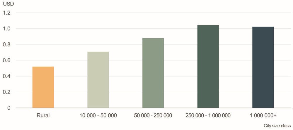
Productivity levels of workers and firms in cities tend to be higher than in rural areas everywhere in the world, which is reflected in higher average wages for workers in urban areas. Africa is no exception to this pattern. Average hourly wages in the six countries for which wage data is available (ETH, MLI, MWI, NGA, TZA and UGA) are USD 0.51 in rural areas and USD 1.03 in medium-large and very large cities, a difference of approximately 100% (Figure 1.2). This wage gap is directly reflected in various measures of living standards, including consumption and wealth measures, but also in other outcomes, such as asset ownership, that are discussed below.
Figure 1.2. Hourly wages in cities and rural areas, 2010
Note: Average based on data for ETH, MLI, MWI, NGA, TZA and UGA from 2010-2019.
Source: OECD/SWAC calculations based on World Bank LSMS (2008-2019[6]) and OECD/SWAC (2018[2]).
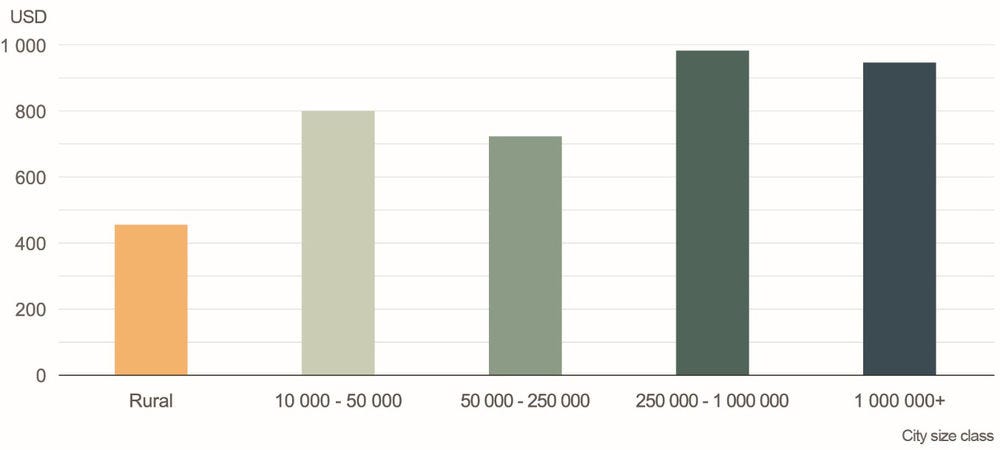
The gap in consumption levels between rural and urban areas is even larger than the gap in hourly wages (Figure 1.3), in particular the gap between small cities and rural areas. Several factors are responsible for this. As discussed below, hours worked are significantly higher in urban areas than in rural areas, which implies that the differences in total wages between rural and urban areas are larger than the differences in hourly wages. Moreover, dependency ratios are lower in urban areas than in rural areas. Per 100 residents of working age, there are roughly 30 fewer residents of non-working age in cities than in rural areas. This implies that a larger percentage of the population in cities is working than in rural areas, which increases average per capita income levels and hence consumption levels for a given wage level.1
Figure 1.3. Annual consumption expenditure in cities and rural areas per capita, 2010
Note: Based on data for ETH, MLI, MWI, NGA, TZA and UGA from 2010-2019.
Source: OECD/SWAC calculations based on World Bank LSMS (2008-2019[6]) and OECD/SWAC (2018[2]).
Box 1.2. How are the key indicators in this chapter calculated?
Most indicators in this chapter are derived from DHS and LSMS microdata that are matched to cities defined by Africapolis (see Box 1.1 for a description of the datasets). The following steps have been used to construct indicators:
1. Individuals and/or households in the DHS and LSMS surveys are matched to the build-up areas of cities as defined by Africapolis, based on their location. This step is complicated by the fact that DHS and LSMS do not use homogenous definitions of urban areas and that they include a random offset of 2 or 5 kilometres in the co-ordinates of household locations, to preserve the anonymity of respondents. To work around this issue, a household is assigned to a city if it is defined by DHS or LSMS as an urban household and if a city according to the Africapolis definition is located within the radius of uncertainty. Likewise, households that are defined by DHS or LSMS as rural but that have a probability greater than 50% of being actually located within the built-up area of a city according to Africapolis are allocated to this city.2 In total, it was possible to match observations from the DHS and LSMS to roughly one-third of the 7 721 cities in the Africapolis database. All remaining households were classified as rural.
2. City-level averages are created by averaging all individuals assigned to the city using the survey weights provided by the DHS and LSMS surveys. This is done separately for each survey wave. Averages for different years are thus created for cities that were covered by multiple survey waves at different points in time.
3. Averages for city-size classes are created by averaging all city-level averages across all available countries within the size class from 2010-2019. Cities are weighted so that each city has the same influence on the city-size class average, no matter by how many surveys it was covered by during the period or how many inhabitants it has. Likewise, averages for rural areas were created by averaging the country average in rural areas for all countries that were covered. The rural area from each country has the same influence on the rural average, no matter how many inhabitants it has.
In contrast to the DHS and LSMS data, firms in Enterprise Surveys are not identified by their location. Instead, the survey data indicates whether a firm is located in a city with between 50 000 to 250 000 inhabitants, between 250 000 and 1 million inhabitants or in a city with more than 1 million inhabitants, often without providing an exact identification of the city. As it is impossible to match firms to individual cities, firms have been averaged by the city-size categories provided by Enterprise Surveys, using the sample weights provided, without further processing.
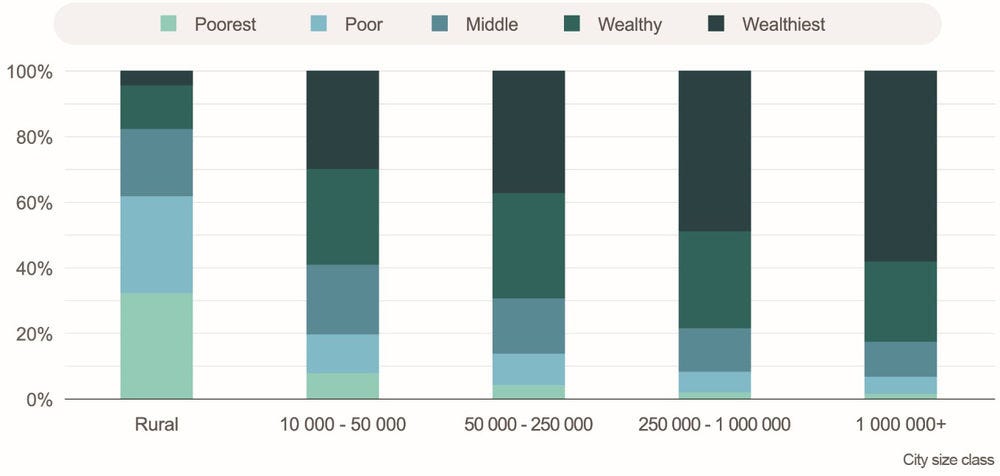
Striking differences between rural and urban areas can also be seen in the wealth distribution. Whereas only 4% of the rural population belongs to the top wealth quintile of a country on average, the share is 30% in cities with between 10 000 and 50 000 inhabitants and increases to 59% in cities with more than 1 million inhabitants. Conversely, the share of residents in the poorest wealth quintile is 33% in rural areas but just 2% in the largest cities of more than 1 million inhabitants (Figure 1.4).3 This wealth gap is reflected in the ownership of specific assets. For example, 18% of residents in cities with more than 1 million inhabitants belong to a household that owns a car, while the corresponding figure in rural areas is just 3%.
Figure 1.4. Share of residents in rural and urban areas by wealth quintile
Note: Based on data from various years between 2010-19 for AGO, BEN, BFA, BDI, CIV, CMR, COD, COM, GAB, GHA, GIN, KEN, LBR, LSO, MDG, MLI, MOZ, MWI, NAM, NGA, RWA, SEN, SLE, TCD, TGO, TZA, UGA, ZAF, ZMB, ZWE. Data on wealth quintiles are obtained from the DHS wealth index.
Source: OECD/SWAC calculations based on ICF (1990-2019[1]) and OECD/SWAC (2018[2]).
As mentioned above, cross-country averages do not reflect the substantial variation between countries. For example, 18% of individuals in large cities live in a household that own a car, but this figure is not representative for many cities. In Cape Town (ZAF), 49% of all households own a car, whereas the corresponding figure is less than 3% in Kisii (KEN) (Figure 1.5).
Figure 1.5. Car and motorcycle ownership rates by cities
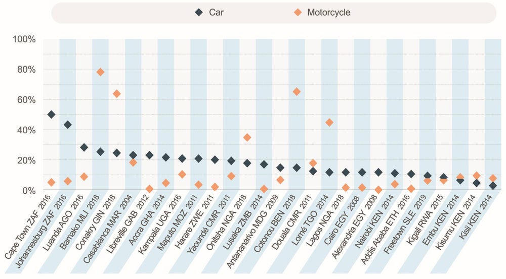
Note: The figure shows the number of individuals living in households that own a car/motorcycle. As household sizes differ across countries, this indicator is not representative of the car/motorcycle ownership per capita. See Box 1.3 for details on how cities in the chart were selected.
Source: OECD/SWAC calculations based on ICF (1990-2019[1]) and OECD/SWAC (2018[2]).
Urban employment rates are lower than in rural areas, but underemployment is less prevalent
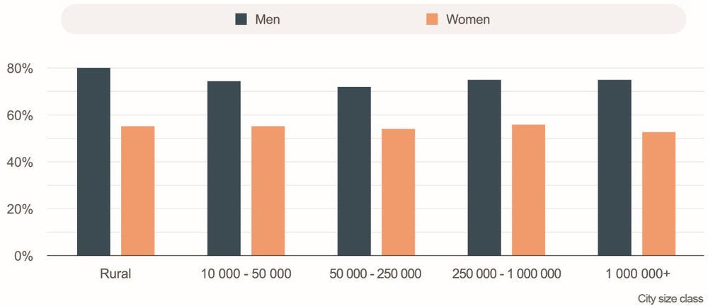
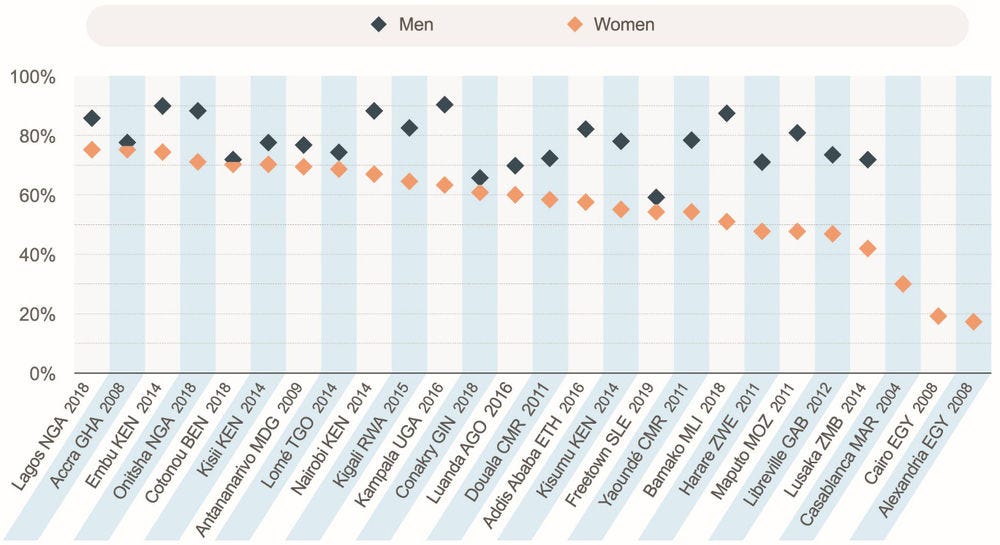
Higher wages in cities do not translate into higher employment rates. Urban employment rates are in fact slightly lower than in rural areas. On average in cities, between 79% and 82% of men (aged 18-49) and 58% to 61% of women (aged 18-49) are in employment. In contrast, 85% of men and 60% of women are employed or self-employed in rural areas (Figure 1.6). Employment rates are generally higher for men than for women, but the differences in cities vary widely across countries. Figure 1.7 shows that North African cities in particular have very low employment rates for women. In other cities, such as Accra (Ghana), Antananarivo (Madagascar) and Lomé (Togo), employment rates for women are nearly as high as for men.
Figure 1.6. Employment rates of individuals aged 18-49
Note: Based on data from various years between 2010-19 for AGO, BEN, BFA, BDI, CIV, CMR, COD, COM, GAB, GHA, GIN, KEN, LBR, LSO, MDG, MLI, MOZ, MWI, NAM, NGA, RWA, SEN, SLE, TCD, TGO, TZA, UGA, ZAF, ZMB, ZWE. Individuals aged 18-49.
Source: OECD/SWAC calculations based on ICF (1990-2019[1]) and OECD/SWAC (2018[2]).
Figure 1.7. Employment rate by gender in selected cities
Note: Individuals aged 18-49.
Source: OECD/SWAC calculations based on ICF (1990-2019[1]) and OECD/SWAC (2018[2]).
Box 1.3. Why are indicators shown only for a few cities?
The procedure described in Box 1.2 makes it possible to match observations from the DHS and LSMS databases to approximately 2 500 cities across Africa. However, in most instances, the number of observations is not sufficient to provide reliable statistics for an individual city, because the DHS and LSMS data was not expressly collected to be analysed at a high degree of geographical disaggregation. Both surveys use cluster sampling, which does not select respondents randomly from all locations. Instead, the sampling locations (so-called sampling clusters) are randomly selected, and all 20 to 30 households at the location are surveyed. As a result, a typical city includes data from 150 individuals (many of them children) from 30 different households in a narrowly defined neighbourhood in the city.
Thus, even if the data contains information on several hundreds of individuals in a city, this may not be sufficient to create reliable averages for the city, because individuals have been sampled from only a few locations within the city. As a consequence, the data for many cities is not representative, because in many instances, mostly poor or mostly rich neighbourhoods happen to have been surveyed. Only if the number of sampling locations is high is it likely that the locations are representative of the city as a whole. To avoid providing a misleading picture, data for individual cities is reported only if at least 500 individuals from 250 households sampled from at least 50 different locations in the city were surveyed. In those cities, it is much less likely for the results to be dependent on the location of the sampling clusters. However, city-level data for all cities will be made available to interested researchers and analysts. To request access to the data, contact africapolis@oecd.org.
Importantly, the sampling error for individual cities is much less of a concern if the data is averaged by city-size class. In this case, the sampling error for individual cities averages out, and the resulting indicators for city-size classes have a much higher accuracy than the indicators for individual cities.
High rural employment rates are counterbalanced by the low number of hours worked
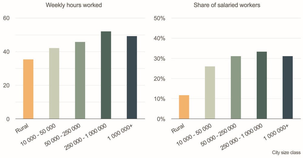
While employment rates in cities are slightly lower than in rural areas, this is more than outweighed by the difference in the number of hours worked. On average, employed rural residents work 36 hours a week, compared to up to 49 hours in cities with more than 1 million inhabitants – a difference of 39%. The high employment rate in rural areas masks significant underemployment, i.e. workers working fewer hours than they could if they had a choice, largely due to the seasonality of agricultural labour. Moreover, the share of salaried workers is significantly higher in larger cities.
Figure 1.8. Urban residents work more hours and are more likely to be salaried
Note: Based on data for ETH, MLI, MWI, NGA, TZA and UGA from 2010-2019.
Source: OECD/SWAC calculations based on World Bank LSMS (2008-2019[6]) and OECD/SWAC (2018[2]).
Box 1.4. The economic impact of COVID on African cities
The COVID-19 pandemic has inflicted a major toll on Africa. Quite apart from the public health impact, which has still not been clearly measured, it has had major economic consequences. Employees in the informal sector, for example, lost 7.7% of their incomes on average due to lockdowns, mostly without receiving any support from social protection programmes (ILO, 2021[8]). The number of Africans threatened by food insecurity has also risen by 60%, to more than 100 million (World Bank, 2021[9]).
The economic downturn has had dramatic consequences for public finances. The pandemic is predicted to reduce Africa’s public revenues by 5%, and city-level governments could lose up to 60% of their revenues in 2021 (UN-Habitat, UNECA, UNCDF and UCLGA, 2020[10]). This decline is especially dramatic in light of the already weak fiscal capacity of local governments prior to the outbreak of pandemic (see Chapters 4 and 5).
As of the time of writing of this report, the pandemic was ongoing and its consequences were not yet fully understood. While it is possible that its economic impact will only be transitory, long-term effects on urban economies, due either to a lasting economic crisis or to changes in urbanisation patterns, cannot be ruled out. For this report, data from up to 2019 have been available. The statistics presented thus do not show the impact of the COVID-19 pandemic.
The share of workers in skilled occupations is higher in cities
Across the world, urban areas have more complex economies than rural areas. Cities in emerging economies are often centres of industrial activity, while cities in advanced economies tend to rely on services. In contrast, rural areas have a much stronger reliance on agriculture and extractive activity and often have lower shares of skilled and service sector jobs. Nevertheless, especially in high-income countries, agriculture tends to employ only a small fraction of individuals, even in rural areas. In the average OECD country, only 7% of all workers in rural areas are employed in agriculture (OECD, 2021[11]).
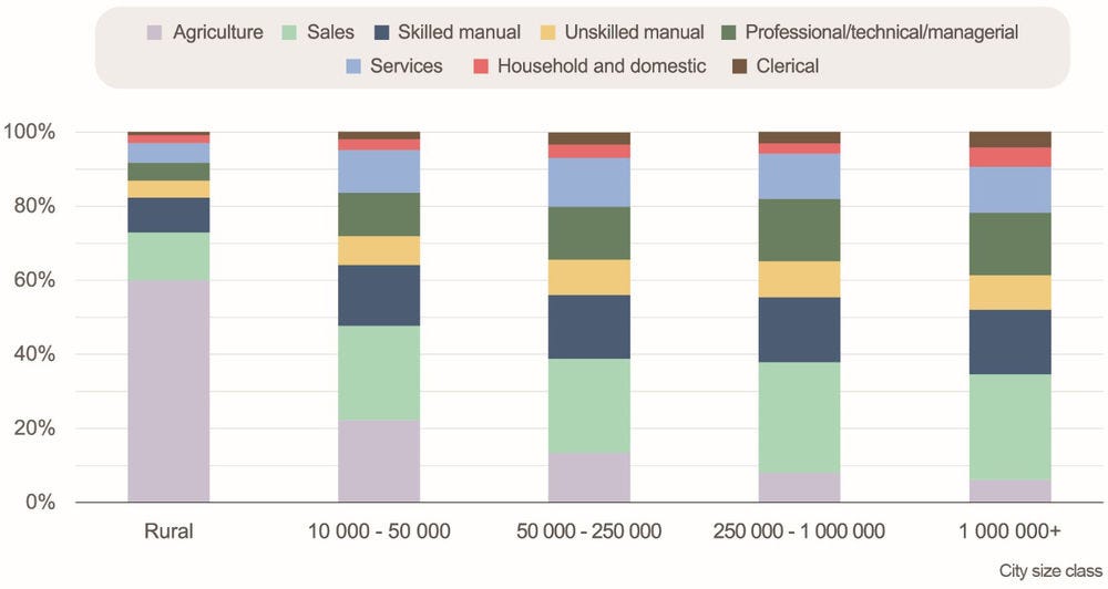
In Africa, agriculture is the dominant occupation in rural areas, at close to 60% of all workers employed. Urbanised countries tend to have somewhat lower rates of agricultural employment. In contrast, sales, skilled manual work, services, and professional, technical and managerial activities are the dominant occupations in cities of all sizes. Together, they make up approximately half of all jobs in urban areas (Figure 1.9). Even in small cities of less than 50 000 inhabitants, only 16% of the workforce are directly employed in agriculture. Of course, this figure does not take into account the indirect importance of agriculture, as a sizeable part of the workforce in these cities is employed in sectors that depend on agriculture, such as the trade or processing of agricultural goods.
Figure 1.9. Composition of the rural and urban economy by sector
Note: Based on DHS surveys from various years between 2010-19 for AGO, BEN, BFA, BDI, CIV, CMR, COD, COM, GAB, GHA, GIN, KEN, LBR, LSO, MDG, MLI, MOZ, MWI, NAM, NGA, RWA, SEN, SLE, TCD, TGO, TZA, UGA, ZAF, ZMB, ZWE.
Source: OECD/SWAC calculations based on ICF (1990-2019[1]) and OECD/SWAC (2018[2]).
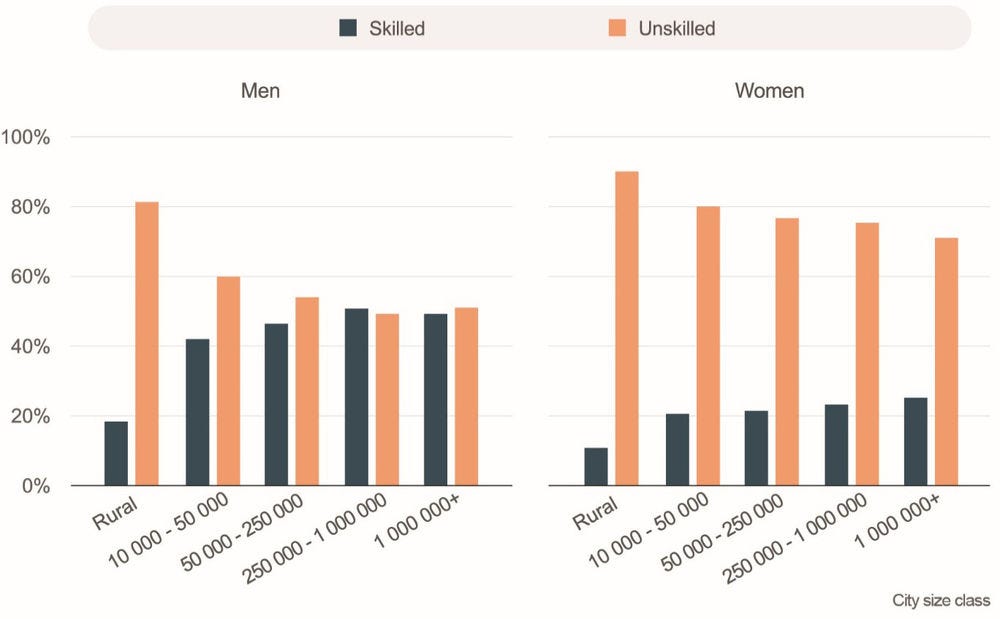
The occupational categories provided by the DHS can be classified in skilled and unskilled occupations. While such a classification is only approximate, given the lack of detail within the available occupational categories, it shows a very clear pattern. The share of skilled occupations is significantly lower in rural areas than in cities. Among men, less than 20% of working individuals work in skilled occupations in rural areas, compared to approximately 50% in midsized and large cities. The share of women in skilled occupations is generally lower, but the pattern is the same: 11% of women are employed in skilled occupations in rural areas, while the share in cities of different sizes ranges from 20% to 25%. Thus, for both genders, the share of skilled workers in large cities is approximately 2.5 times that in rural areas.
Figure 1.10. Share of workers in skilled and unskilled occupations
Note: Based on DHS surveys from various years between 2010-19 for AGO, BEN, BFA, BDI, CIV, CMR, COD, COM, GAB, GHA, GIN, KEN, LBR, LSO, MDG, MLI, MOZ, MWI, NAM, NGA, RWA, SEN, SLE, TCD, TGO, TZA, UGA, ZAF, ZMB, ZWE. Occupational categories provided by DHS have been classified into skilled/unskilled as follows. Skilled occupations are defined as professional, technical, managerial, clerical and skilled manual work. Unskilled occupations are defined as sales, agriculture, household and domestic work, services, and unskilled manual work.
Source: OECD/SWAC calculations based on ICF (1990-2019[1]) and OECD/SWAC (2018[2]).
Figure 1.11 shows the relationship between the share of skilled jobs and the urban/rural status by country. While country-level estimates necessarily have a higher sampling noise and are therefore less precise than aggregate numbers, it is notable that the pattern described above holds in most countries.
Figure 1.11. Share of workers in skilled occupations by country and city-size class
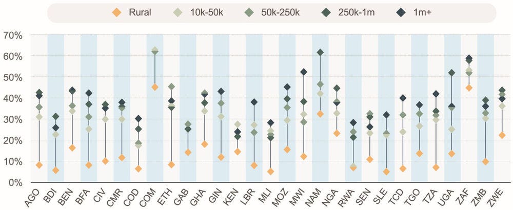
Note: Data for various years from 2010-19. Occupational categories provided by DHS have been classified into skilled/unskilled. Skilled occupations are defined as professional, technical, managerial, clerical and skilled manual work. Unskilled occupations are defined as sales, agriculture, household and domestic services, and unskilled manual work.
Source: OECD/SWAC calculations based on ICF (1990-2019[1]) and OECD/SWAC (2018[2]).
Education levels in cities are higher than in rural areas
The higher share of skilled jobs in cities can – at least partly – be explained by the higher education levels. Whereas on average 42% of the population in rural areas in the covered countries does not have any formal education, the share is only 13% in large cities. Likewise, the number of average years of schooling varies from 4 years for women in rural areas to almost 10 years for men in large cities. Notably, the gender gap is somewhat smaller in large cities, indicating that urbanisation has benefits for female education. Importantly, these numbers refer to the entire population above age 18 and older and not to current graduates. As noted below, education levels in Africa are rising across rural and urban areas alike. Average education levels in the general population are thus lower than average education levels of young adults.
Figure 1.12. Education levels in rural areas and cities
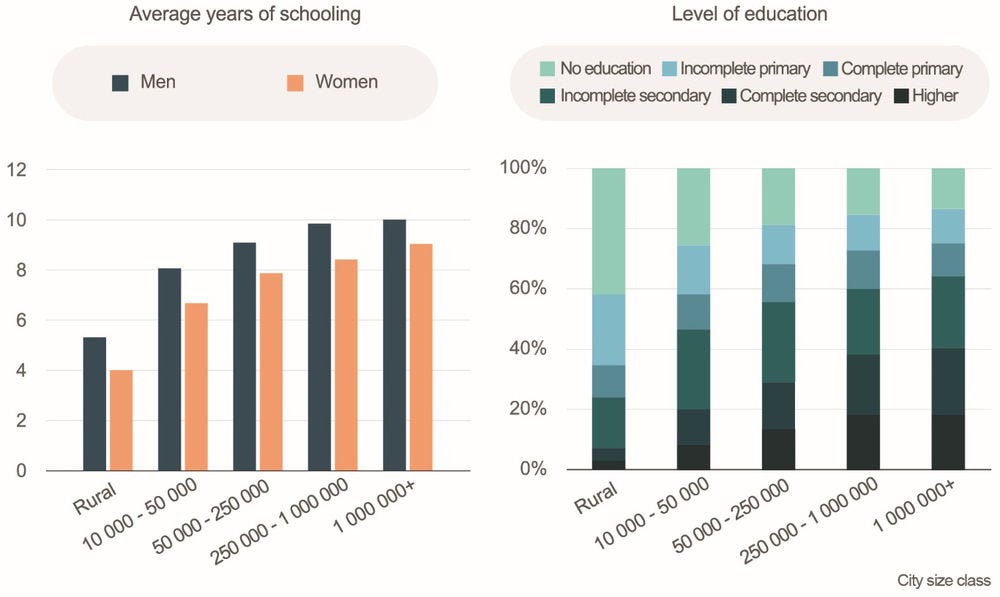
Note: Based on DHS surveys from various years between 2010-19 for AGO, BEN, BFA, BDI, CIV, CMR, COD, COM, GAB, GHA, GIN, KEN, LBR, LSO, MDG, MLI, MOZ, MWI, NAM, NGA, RWA, SEN, SLE, TCD, TGO, TZA, UGA, ZAF, ZMB, ZWE. Respondents aged 18 and older.
Source: OECD/SWAC calculations based on ICF (1990-2019[1]) and OECD/SWAC (2018[2]).
Cities attract educated people everywhere in the world. Thus, the difference in education levels could be due to the fact that more educated people tend to move to cities. However, the data do not support this hypothesis. Although rural-urban migrants aged 18-29 who move to cities at age 18 or older have on average 3 to 3.5 years more education than their rural peers of the same age who have never moved, they still tend to be less educated than urban residents aged 18-29 who grew up in a city. For all city-size classes, the education level of residents born there who have never moved is higher than the education level of rural-born residents who moved there at age 18 or older. The large gaps in education levels between cities and rural areas are thus not primarily due to selective migration, but to the easier access to education in cities and the greater importance of education in an urban economy.
The boost to education that urbanisation affords is arguably one of its most important benefits. Education has major positive influences on job opportunities, health outcomes and other dimensions of well-being over the course of a person’s lifetime (OECD, 2021[12]), meaning that the economic and social benefits will persist over many decades. This also implies that many of the economic benefits of the higher levels of education that children in African cities receive today will materialise only in the years to come.
Despite the benefits cities offer in providing access to education, it is important to emphasise that some cities do better than others. Figure 1.13 shows that large differences in education levels exist across cities of different sizes. Some cities are much more successful in providing secondary education to their residents and have shares of the population with secondary education that easily exceed 50%, while the share remains below 20% in other cities. As similarly diverse sets of outcomes can be found across many dimensions, it is a reminder that public policies matter and that the benefits of urbanisation do not materialise automatically.
Figure 1.13. Share of residents with secondary or higher education
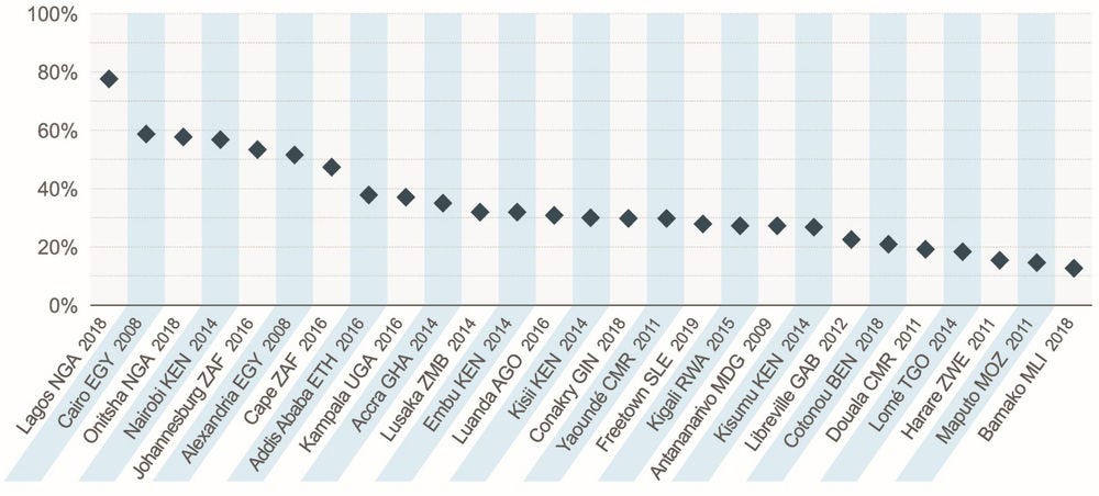
Note: Respondents aged 18 and older.
Source: OECD/SWAC calculations based on ICF (1990-2019[1]) and OECD/SWAC (2018[2])
Firms in cities are more innovative
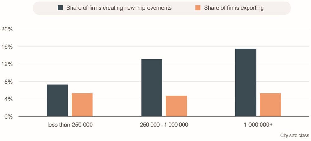
Firms in larger cities are more likely to be engaged in innovative activities, such as creating new products or improvements (Figure 1.14). In small to medium-sized cities with fewer than 250 000 inhabitants, approximately 8% of firms develop new improvements to products, whereas the share is twice as high in cities with more than 1 million inhabitants. As innovation is the key driver of productivity growth, the increased innovative activity contributes to higher levels of productivity in larger cities.
Even though international evidence suggest that innovative firms export more (Bustos, 2011[13]) and that larger cities rely disproportionally on exports (Marin et al., 2020[14]), this pattern is not reflected in city-level data in Africa (Figure 1.14). Potentially, this is due to the outsized importance that the export of raw materials has in the export portfolio of African economies. As the producers of raw materials are likely to be located in rural areas and smaller cities, they counteract the export-enhancing effect of greater innovative activity in large cities.
Figure 1.14. Innovation and export activity of firms by city size
Moreover, compared to cities with less than 250 000 inhabitants, firms in cities with between 250 000 and 1 million inhabitants have a share of employees with secondary education 7 percentage points higher and firms in cities of above 1 million inhabitants have a share 11 percentage points higher. This corresponds to the result noted earlier that the share of skilled jobs is higher in larger cities than in smaller ones.
Infrastructure provision is more efficient in cities
Cities across the globe have higher levels of infrastructure than rural areas because infrastructure can be provided more efficiently to urban residents than to rural residents. Because of higher population densities, more people can benefit from a given infrastructure investment in a city than in a rural area. This makes it cheaper to provide infrastructure to city dwellers than to rural populations. Likewise, the provision of other essential infrastructure, such as transport and telecommunications infrastructure, is cheaper on a per capita basis in cities than in rural areas. High densities of people and firms in cities also allows the provision of infrastructure that would not be viable in rural areas, such as metro systems, airports and various forms of specialised industrial infrastructure, such as high-throughput data cables. Workers and firms become more productive because they benefit from this infrastructure.
In Africa, infrastructure levels between cities and rural areas differ substantially, which is reflected in the share of households that have access to electricity, piped water and telecommunications networks. The differences are most pronounced with respect to electricity provision. Less than 20% of households in rural areas have access to electricity, while the share reaches 58% in small cities with less than 50 000 inhabitants and 80% in cities with more than 1 million inhabitants. Access to piped water on the plot is generally much less widespread and varies from 7% in rural areas to 25% in small cities and 33% in large cities.4 In contrast, mobile phone coverage and ownership is widespread, with 63% of households owning a mobile phone in rural areas, 85% in small cities and 94% in large cities.
Notably, the gap between rural areas and cities (of any size) is much larger than the gap between small and large cities. The differences between rural areas and small cities in the share of households that have access to electricity, water and mobile phones, respectively, are approximately twice as large as the differences between small cities and large cities. This pattern holds for many other outcomes analysed in this chapter.
Figure 1.15. Access to public utilities
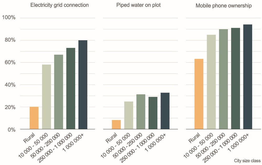
Note: Based on DHS surveys from various years between 2010-19 for AGO, BEN, BFA, BDI, CIV, CMR, COD, COM, GAB, GHA, GIN, KEN, LBR, LSO, MDG, MLI, MOZ, MWI, NAM, NGA, RWA, SEN, SLE, TCD, TGO, TZA, UGA, ZAF, ZMB, ZWE.
Source: OECD/SWAC calculations based on ICF (1990-2019[1]) and OECD/SWAC (2018[2]).
It is important to keep in mind that Figure 1.15 shows the general differences across rural areas and cities of different sizes, but it is not representative of individual countries. A breakdown of access to electricity by city-size class and country (Figure 1.16) shows that majorities of households in large and midsized cities have access to electricity. In contrast, electrification rates in small cities vary strongly across countries, while rural electrification rates are below 50% in most countries.
Figure 1.16. Share of households with access to electricity by country and city size
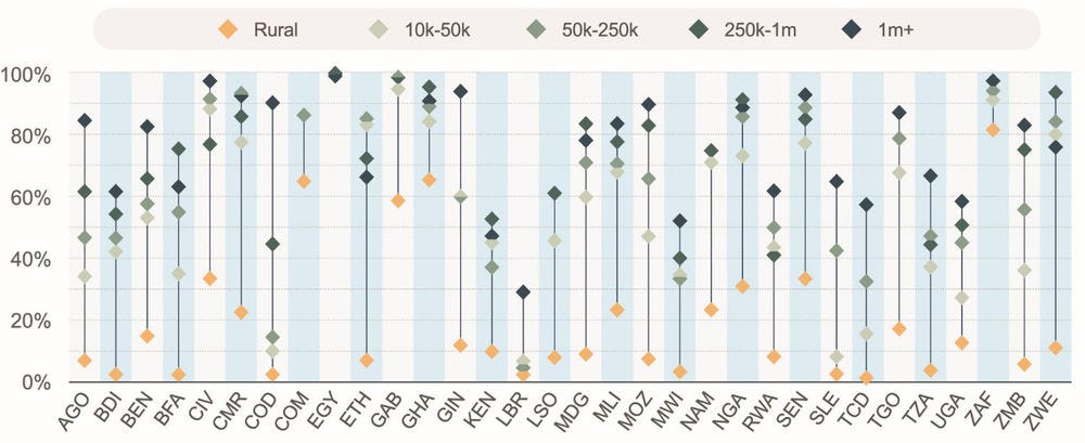
Note: Data for various years between 2010 and 2019 and Egypt 2008.
Source: OECD/SWAC calculations based on ICF (1990-2019[1]) and OECD/SWAC (2018[2])
Access to piped water on the plot varies even more strongly across countries. Figure 1.17 shows the share of population with access to electricity and water for selected cities. Whereas electricity access is widespread in almost all large cities, access to piped water on the plot varies strongly across cities. While more than 80% of residents in Addis Ababa (Ethiopia) have piped water access on their plot, the share is just slightly above 10% in Accra (Ghana). Similar differences can be found across cities of all sizes.
Figure 1.17. Share of residents with electricity and private piped water access in selected cities
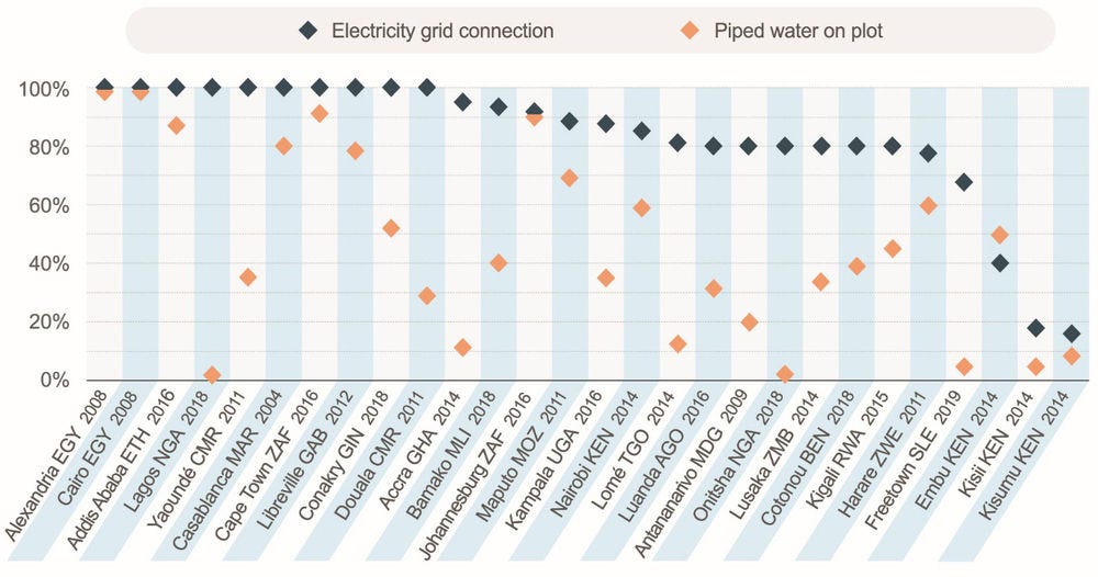
Note: Lagos stands out as one of Africa’s largest cities that also has one of the lowest rates of access to piped water, since 33% of households obtain their water from private boreholes, and 57% from water sachets (i.e. water packaged into small plastic bags). See Danert and Healy (2021[15]) and National Population Commission and ICF (2019[16]) for further details.
Source: OECD/SWAC calculations based on ICF (1990-2019[1]) and OECD/SWAC (2018[2]).
Pillars of the formal economy are more developed in cities
The available data do not allow for measuring the scale of the formal and informal economy in rural and urban areas. However, urban areas are more likely to meet many of the preconditions to facilitate a transition to the formal economy. The share of individuals that own a bank account is 2 to 3 times higher in cities of different sizes than in rural areas. Likewise, close to half of all individuals own a title to their house in urban areas, while the share is less than 20% in rural areas. Urban residents are also more likely to have a birth certificate or to be registered with the public administration, even if the gap is small compared to the previous outcomes. While none of these factors alone is sufficient to enable a transition to the formal economy, the absence of any of them can create a bottleneck that prevents such a transition.
Figure 1.18. Share of residents in households with bank accounts, with titles to their house and birth certificates
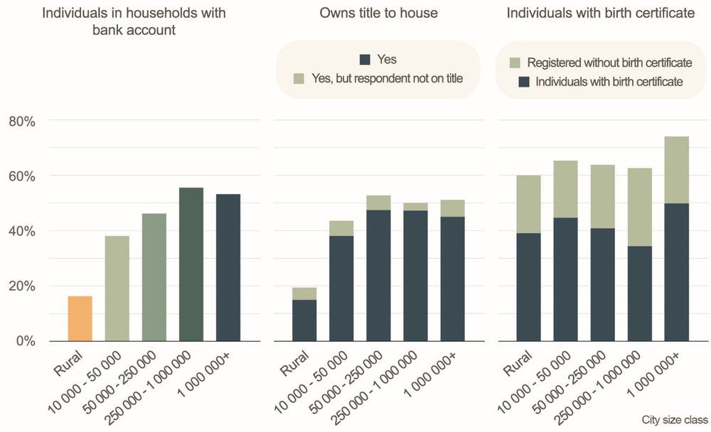
Note: Based on DHS surveys from various years between 2010-19 for AGO, BEN, BFA, BDI, CIV, CMR, COD, COM, GAB, GHA, GIN, KEN, LBR, LSO, MDG, MLI, MOZ, MWI, NAM, NGA, RWA, SEN, SLE, TCD, TGO, TZA, UGA, ZAF, ZMB, ZWE.
Source: OECD/SWAC calculations based on ICF (1990-2019[1]) and OECD/SWAC (2018[2]).
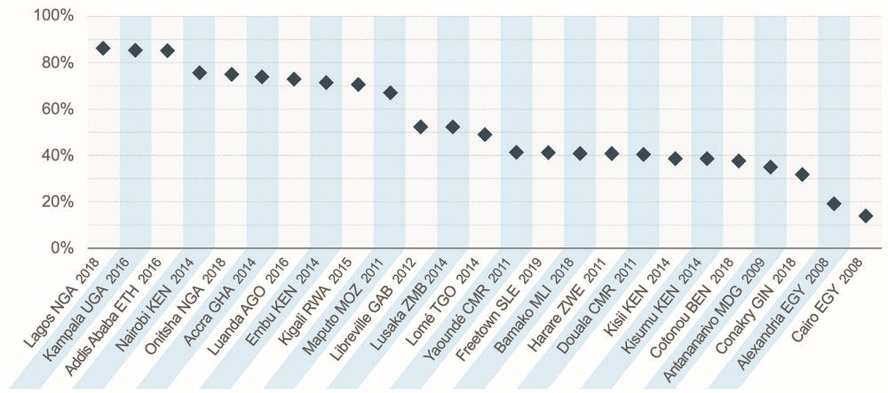
Mobile banking has made banking services available to large groups of people who did not previously have access to financial institutions. Figure 1.18 presents an average for the years 2010-2019, the share of residents in households with a bank account is probably an underestimation of today’s value. As Figure 1.19 shows, more than 80% of residents live in households that have a bank account in 2016 and 2018 in major African cities such as Lagos (NGA), Kampala (UGA) and Addis Ababa (ETH). Nevertheless, there are still large cities, such as Conakry (GIN), where less than a third of residents live in a household that has a bank account.
Figure 1.19. Share of residents that live in households with a bank account
Dependency ratios and fertility rates are lower in cities
Africa has by far the highest dependency ratio of any global region. In 2015, on average, 100 working age people (aged 15-64) had to support 80 non-working age people. In contrast, dependency ratios in other global regions vary from 47 to 55 non-working age people per 100 working age people (UNDESA, 2019[17]). The high dependency ratio is mostly due to a high birth rate. More than 90% of the dependent population in Africa are children, whereas up to half of the dependent population in other parts of the world consists of the elderly.
Lower dependency ratios increase per capita GDP levels and improve living standards because the output produced by the working population has to be shared among a smaller non-working population. Assuming a constant employment rate and constant labour productivity, a decrease in the dependency ratio from 80 to the global average of approximately 50, would increase per capita GDP by 20%. Dependency ratios could decrease further, because high child dependency ratios carry the seeds of a demographic dividend. If fertility rates decline to replacement levels (approximately 2.1 births per woman), countries can quickly move from disproportionally high dependency ratios to disproportionally low dependency ratios, because the decline in fertility is quickly reflected in lower child dependency ratios, while it takes decades until it is reflected in higher old-age dependency ratios.
In the 32 countries for which data exists, total fertility rates in large cities averaged 3.7 births per women between 2010 and 2019, as opposed to 5.9 in rural areas (Figure 1.20 left panel). Across all of Africa, total fertility rates have declined from 6.2 in 1990 to 4.4 in 2020 (UNDESA, 2019[17]). This downward trend occurred relatively uniformly across rural areas and cities of any sizes, and the gap between rural areas and cities remained relatively constant over time. While the fertility rate is the most important determinant of dependency ratios, they are also affected by rural-urban migration. The large gap in dependency ratios between rural areas and small cities with between 10 000 and 50 000 inhabitants (Figure 1.20 left panel) that is not reflected in fertility rates could be an indication that rural-urban migrants into these cities do not take their children with them (perhaps because they are located close to their rural homes). However, further investigations would be necessary to confirm this hypothesis.
Figure 1.20. Dependency ratio and fertility rates in rural and urban areas
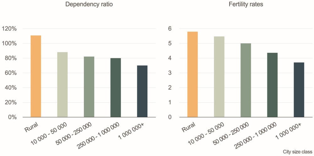
Note: Based on DHS surveys from various years between 2010-19 for AGO, BEN, BFA, BDI, CIV, CMR, COD, COM, GAB, GHA, GIN, KEN, LBR, LSO, MDG, MLI, MOZ, MWI, NAM, NGA, RWA, SEN, SLE, TCD, TGO, TZA, UGA, ZAF, ZMB, ZWE. Diverging from the description in Box 1.2, the data were constructed by averaging all observations belonging to a city-size class within a DHS survey without first averaging by city.
Source: OECD/SWAC calculations based on ICF (1990-2019[1]) and OECD/SWAC (2018[2]).
Small and midsized cities perform well
One of the most notable patterns in the data presented above is the good performance of small and midsized cities. Even small cities perform notably better than rural areas along almost all measurable outcomes. While they tend to perform worse than larger cities, the gap between small and large cities is usually much smaller than the gap between rural areas and small cities.
These results indicate that in many cases, certain minimum sizes or minimum population densities are required for an economic activity, a public service or an infrastructure provision. Once the required threshold is exceeded, any additional population does little to facilitate the economic activity or service or infrastructure provision further. For example, almost any city of 10 000 inhabitants will have enough students to allow for the efficient operation of a secondary school. While larger cities might allow for more specialised secondary schools or a larger choice of secondary schools, these gains tend to be small relative to the benefit that comes from exceeding the necessary population size that allows for the operation of a secondary school. Similar threshold effects might occur with respect to many other outcomes, such as the viability to have a specialised market or a bank branch in a city.
Of course, not all benefits of urbanisation occur at certain thresholds. Some benefits of urbanisation continue to accumulate with increasing city sizes and population densities. For example, larger cities tend to have more complex economies because they allow for more specialised economic activities. This complexity increases with city size, without depending on any obvious thresholds.
Averages hide substantial variation across and within cities
This chapter presents primarily averages by city-size class to show the typical patterns that can be found across Africa. Although such averages are meaningful and important, they only present a partial picture because they cannot reflect the substantial variation that exists across and within cities. As discussed above, large differences exist between cities, with many cities performing well in some dimensions, but not in others. Within cities, differences between poor and wealthy residents are even larger than average differences across cities. Due to the lack of suitable data, this report does not discuss the gap between the formal and informal sector. The statistics presented generally cover both sectors, even though economic and social conditions tend to be much more favourable in the formal than in the informal sector. Likewise, the place of residence within a city has major consequences on living standards. Slum dwellers often have much poorer access to services and infrastructure than individuals living in formal housing. Again, these differences have not been discussed in detail, given the lack of cross-country data that would permit a rigorous quantitative analysis.
Estimating GDP gains from urbanisation
Most cities generate significant agglomeration economies (OECD, 2015[18]). The term agglomeration economies describes a set of factors that increase productivity, wages and innovation when economic activity is located in close geographical proximity (Box 1.5). Cities, and especially large cities, are the main beneficiaries of agglomeration economies, because of the high density of their economic activity.
Africa’s cities have higher productivity levels than rural areas, and larger cities have higher productivity levels than smaller cities. This is reflected in higher wages (Figure 1.2) and higher GDP levels. While this pattern suggests that urbanisation contributes to better economic outcomes, it is not conclusive evidence. A possible alternative explanation could be that cities and especially large cities attract particularly productive workers or industries and advanced industries, a process that economists call sorting. If sorting were the only explanation for the good performance of cities, urbanisation would not benefit national economies, as the productive workers and industries that locate in cities would be equally productive if they remained in rural areas. Under this explanation, urbanisation would only affect where productive firms and workers are located, but it would not add to overall productivity levels across the national economy.
Sorting of workers and firms is common in most countries, including in Africa. As noted above, rural-urban migrants have on average 3 to 3.5 years more of education than rural residents of comparable age who do not move to cities. On average, an increase in city size by 10% is correlated with a 0.3 percentage point higher share of workers in skilled occupations. Figure 1.21 breaks down the relationship between city size and share of skilled job by country. For each country, it shows the estimated increase in the share of skilled jobs in response to a 10% increase in city size, as well as the 95% confidence interval for the estimate. For most countries, the estimated coefficient falls between 0.1 and 0.6, meaning that the share of skilled workers increases on average by 0.1 to 0.6 percentage points if the size of a city increases by 10%.
Figure 1.21. Percentage point increase of skilled jobs in response to a 10% increase in city size
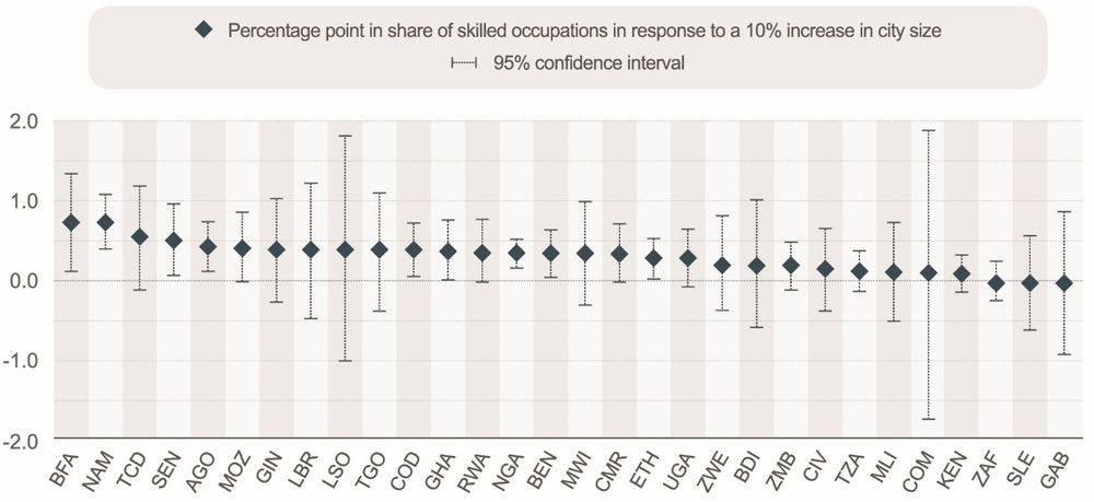
Note: Estimated increase in the share of skilled jobs in a city if city size increases by 10%. Occupational categories provided by DHS have been classified into skilled/unskilled. Skilled occupations are defined as professional, technical, managerial, clerical and skilled manual work. Unskilled occupations are defined as sales, agriculture, household and domestic services, and unskilled manual work. See Annex Table 1.A.2 for details on the estimated specification.
Source: OECD/SWAC calculations based on ICF (1990-2019[1]) and OECD/SWAC (2018[2]).
Yet, high levels of productivity in cities are not only due to sorting. Even when controlling for the education level of workers, their personal characteristics, such as age and sex, as well as the characteristics of the industries in which they work, workers in large cities are more productive than workers in small cities, who in turn are more productive than workers in rural areas (Annex Table 1.A.8 and Annex Table 1.A.7). Thus, the data suggest that cities in Africa generate agglomeration economies just as cities in other parts of the world do.
Box 1.5. What are agglomeration economies?
Agglomeration economies describe a set of factors that increase productivity, wages and innovation when economic activity is located in close geographical proximity to each other. Cities and especially large cities are the main beneficiaries from agglomeration economies because of the high density of economic activity that they host. Most empirical studies typically find that a 10% increase in population size or population density leads to a 0.2%-0.5% increase in productivity, with the most reliable estimates often falling at the lower end of this range (Combes and Gobillon, 2015[19]). In a meta-analysis of 70 studies from developing countries, Grover, Lall and Timmis (2021[20]) conclude that the magnitude of agglomeration economies in low- and middle-income countries is roughly similar and if anything, slightly higher than in high-income countries.
The driving forces behind agglomeration economies have already been discussed by Marshall (1890[21]), who highlighted three mechanisms that are still considered to be among the most important: sharing, matching and learning (Puga, 2010[22]). Beyond those, other explanations have been proposed and the issue is still being actively researched.
Sharing
The larger a city, the more potential users for a service or an infrastructure exist. This makes it possible in large cities to provide public or private services and infrastructure that are not viable in smaller cities. Businesses that have access to them can operate more productively than businesses that do not. For example, in a large city, a privately run industrial park targeted to the chemical industry can be viable. Among other services, the park might offer a pipeline system to provide various commonly needed industrial gases to client firms that locate within the park. A chemical firm located within the park could thus operate more productively than a similar chemical firm in a small city or rural area that does not have access to a similar system and needs to ship those gases by truck.
Beyond sharing access to services and infrastructure, firms may also share a network of suppliers, thereby having access to more specialised inputs, which also raises productivity.
Matching
In large cities, workers have access to a large number of potential jobs, and employers can choose from a large number of potential applicants. This makes it more likely that a worker finds a position that uses his or her skills to the best possible degree and that firms will find an applicant who has exactly the skills required. For example, a construction worker might have acquired training in an advanced welding technique that is needed only infrequently. In a rural area or a small city, it is unlikely that he or she would find a position that frequently requires such welding skills. The worker would most likely work for a small construction firm and use his or her specialised skills only infrequently. However, in a large city, the chances are higher that the worker could find a job specialised in the welding technique, for example with a large construction firm. In this case, the worker would be able to use his or her specialised skill more frequently and would work more productively than in rural areas.
Learning
Firms and workers become more productive by imitating the approaches of successful competitors and colleagues. As the number of firms and workers in cities is larger than in rural areas, the potential to learn from each other is larger, too. For example, a worker in a large city is likely to encounter many slightly different approaches to the same task, because he or she might speak to colleagues in other firms, work for several firms over the course of a career or observe other firms while working. Some of these approaches will be more efficient than others and the worker is likely to learn from those that work best, thus raising his or her productivity. In smaller cities and rural areas, where fewer similar jobs exist, the potential for learning is limited.
Beyond these sources of externalities discussed by Marshall (1890[21]), another important source has been highlighted by Jacobs (1969[23]). Cities generate innovation because a large number of people from different professions meet. In these interactions, new ideas are created from existing knowledge. As many innovations tend to spread locally first, they benefit in particular the cities in which they were invented.
Urbanisation has generated almost a third of Africa’s per capita GDP growth since 2020
If the magnitude of agglomeration economies is known, it is possible to conduct back-of-the-envelope estimates of how urbanisation affects GDP. The key measure of agglomeration economies is the so-called city-size elasticity of productivity. This indicates by how much productivity increases if city size increases. To estimate the GDP effect of urbanisation in Africa, average city-size elasticities for five African countries (Ethiopia, Malawi, Nigeria, Tanzania, and Uganda) have been obtained (see Box 1.6). On average, labour productivity5 is estimated to increase by 0.3% if the urban population increases by 10% (see Specification 2 Annex Table 1.A.7). These numbers can be applied to the observed growth of urban and rural areas in order to get a first-order approximation of the consequences for GDP.
Across Africa, the current urbanisation process contributes 0.33 percentage points annually to per capita GDP growth, even without taking into account additional long-run and second-order benefits from urbanisation (e.g. due to the better education that children in cities receive). This is 29% of the total average annual per capita GDP growth across Africa between 2001 and 2020. Thus, even if second-round effects from higher education levels obtained by rural residents are not considered, urbanisation provides a significant contribution to Africa’s per capita GDP growth.
The effect of urbanisation on GDP can be divided into two components. First, the share of the population that lives in more productive urban areas instead of in less productive rural areas increases due to urbanisation. This shift in population distributions increases national GDP levels and hence average per capita GDP. Second, cities become more productive due to the inflow of additional workers, because larger cities have higher productivity levels than smaller ones. In terms of magnitude, the first component contributes approximately two-thirds, while the second component contributes approximately one-third to the predicted per capita GDP growth. The growing share of people living in more productive cities increases per capita GDP by 0.22 percentage points, while cities becoming more productive due to their larger size adds 0.11 percentage points.6
Several important caveats must be noted. On an econometric level, the estimated magnitude of agglomeration economies is subject to considerable uncertainty, due to the conceptual issues discussed in Box 1.6 and due to statistical noise. The city-size elasticity of productivity of 0.03 that is used for the back-of-the-envelope estimate is at the lower end of comparable estimates for developing countries (see Gover, Lall and Timmis (2021[20])). For comparison, if the city-size elasticity was twice as high (an estimate that would fall at the upper end of range of estimates in Gover, Lall and Timmis (2021[20]), the contribution of urbanisation to annual per capita GDP growth would be 0.56 percentage points, or 50% of total average annual per capita GDP growth between 2001 and 2020.
On a conceptual level, it is impossible to capture all consequences of urbanisation. The estimates provide only the GDP effect from productivity gains due to agglomeration economies. They do not take into account other consequences of urbanisation, for example the fact that it causes structural changes to the economy or that it changes the characteristics of the workforce (e.g. because children in urban areas receive more education than in rural areas). Moreover, the estimates only focus on productivity and do not take into account negative externalities from urban growth, such as increasing congestion or exposure to pollution. Thus, the estimates obviously do not capture the full impact of urbanisation, especially over longer time horizons.
Taken together, these caveats imply that the estimates above can at most provide a ballpark range of the medium-term economic gains from urbanisation. They should not be considered precise predictions, nor should they be seen as reflecting all the economic and social processes that are induced by urbanisation. It seems likely that the numbers above underestimate the long-term benefits of urbanisation, in particular in light of the significantly higher levels of education that urban residents receive compared to rural residents. These educational benefits will affect African economies for many decades, but their impact is hard to capture.
Box 1.6. Estimating agglomeration economies in Africa
Several approaches have been developed to estimate agglomeration economies (see Combes, Duranton and Gobillon (2010[24]) for an overview). All have in common that they require large and detailed data on firms and/or workers. The most common approach following Combes, Duranton and Gobillon (2008[25]) uses individual-level data of workers, for example from labour force surveys, to estimate the relationship between productivity and city size. In a first step, city fixed effects of productivity are estimated while controlling for a variety of factors, including worker characteristics (e.g. age, sex, education) and worker fixed effects, occupation and industry. In a second step, the predicted city fixed effects are regressed on population size or density, potentially using an instrumental variable strategy to obtain exogenous variation in those factors.
The only cross-country individual-level dataset containing the required information for Africa is the LSMS data discussed in Box 1.1. Compared to data sources typically used to estimate agglomeration economies, such as labour force surveys, it has several limitations, including a lower number of observations, less detailed information on occupations and industries, and less precise measures of key variables, such as wages. Despite these drawbacks, the data offers the possibility of estimating agglomeration economies in the spirit of Combes, Duranton and Gobillon (2008[25]) if it is matched to urban areas, as discussed in Box 1.2.
Several simplifications have to be made, by comparison with Combes, Duranton and Gobillon (2008[25]) to deal with limitations in the data that is available. First, information on workers is limited by the information available in the LSMS data, and it is not possible to include worker fixed effects in the estimation. The number of individuals in the data who move from one place to another is too low to identify city fixed effects. Second, a single-stage specification is employed rather than a two-stage approach, because it yields more stable results, given the low number of observations. Third, because few data are available on Africa’s cities, area covariates are limited to a few geographical indicators.
Given these limitations, two main specifications are estimated. Annex Table 1.A.8 shows estimates of the productivity differentials by city-size class for all observations, using rural observations as a baseline. Annex Table 1.A.7 provides estimates of city-size elasticities using only urban observations. All observations are weighted so that each city receives equal weight in the estimates.
Box 1.7. Assumptions made to approximate the effect of urbanisation on GDP
To approximate the effect of urbanisation on GDP based on city-size elasticities of productivity, a number of assumptions have to be made. The following assumptions are used.
The population of each city grows according to the observed annual population growth rate between 2000 and 2010. If a city did not exist in 2000, it is assumed to grow at the average growth rate of cities, that is, 3.5%. Rural populations of each country are assumed to grow at the average annual growth rate of the rural population of the respective country in 2000 and 2010.7
All urban population growth takes place within existing cities. No new cities emerge, and cities do not merge with each other.
Cities with 10 000 inhabitants have 18% higher productivity levels than rural areas. This is a conservative approximation, based on the estimates in Annex Table 1.A.8, which indicate that cities with between 10 000 and 50 000 inhabitants have a 21% higher productivity level when controlling for individual and firm-level characteristics.
From a population size of 10 000 onwards, the city-size elasticity of productivity is 0.03, as estimated in Specification 2 in Annex Table 1.A.7. In other words, if a city grows by 10% in population its productivity increases by 0.3%. Rural productivity remains constant.
Changes in labour productivity translate one-to-one into per capita GDP changes.8
Based on these assumptions, per capita GDP levels relative to rural areas for cities of any size any size can be estimated. Once these are known, it is straightforward to obtain total GDP levels with and without population growth and estimate the average per capita GDP growth caused by the abovementioned urban and rural population growth. Since the estimates are scale-invariant, it does not matter which initial GDP level is assumed. The predicted growth rate will always be the same.
Cities have maintained their relative advantage, despite tripling in size since 1990
One of the most under-appreciated achievements of African cities over the last 30 years has been their consistently better performance compared to rural areas, despite absorbing large numbers of rural-urban migrants. In 1990, 3 300 cities with an average of 57 000 inhabitants existed in Africa. By 2015, those cities had grown to more than 140 000 inhabitants on average, and they probably attained an average population of 170 000 in 2020. In addition, another 4 900 cities with an average population of 22 000 inhabitants emerged during this period. Throughout this phase of extremely rapid population growth, cities managed to maintain their above-average performance. Since 1990, they have had a consistently higher share of skilled jobs, higher wealth levels and better infrastructure. If an indicator changed at the national level, the respective trends in rural and urban areas usually moved in parallel.
Figure 1.22 shows the evolution in the share of residents with electricity grid connection, piped water on the plot, the average years of schooling and the share of residents in households with a bank account. Three of the four outcomes show a clear upward trend across all territories, with larger cities mostly preserving their advantage over smaller cities and rural areas. An exception to the largely positive development is access to piped water. The share of residents in households that have access to piped water on their plot declined strongly in cities in the late 1990s and early 2000s. However, it has stabilised since then, and has remained constant, even as cities continued to grow strongly.
Figure 1.22. Performance of key outcomes in cities and rural areas over time
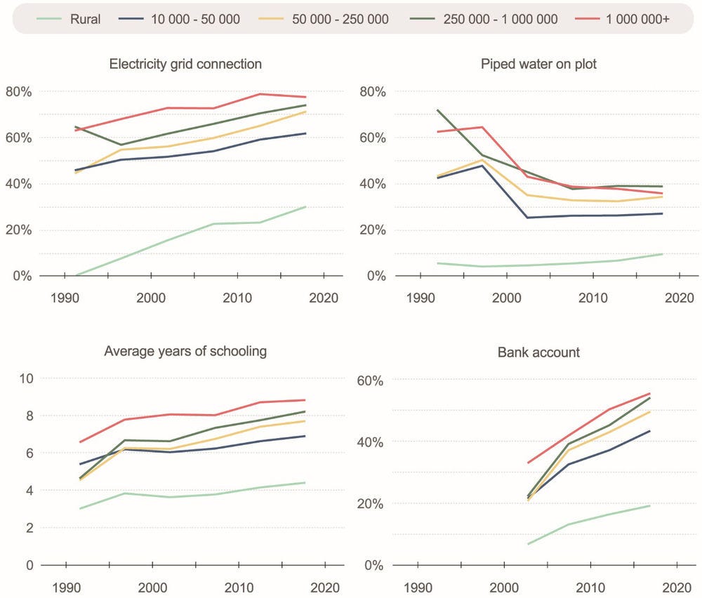
Note: Time trends have been constructed by de-meaning city-level estimates from individual DHS surveys with the respective country average across all DHS surveys, to take into account the fact that the set of countries surveyed by the DHS varies from year to year. To obtain meaningful values on the vertical axis, the average across DHS surveys from all countries and years has been added. Finally, annual averages for city-size classes have been averaged into five-year bins (1990-94, 1995-99, 2000-04, 2005-09, 2010-14, 2015-19) to reduce noise.
Source: OECD/SWAC calculations based on ICF (1990-2019[1]) and OECD/SWAC (2018[2]).
An implication of this stable pattern is that urbanisation benefited economic growth and improved living standards. Even if the relative performance of cities has remained constant, urbanisation has made a major contribution to an increase in living standards. Cities were able to absorb rural migrants as well as natural population growth, and to continue to perform well in their national context. As the urban population increased from less than 190 million people in 1990 to 570 million people in 2015 and approximately 700 million people in 2020, the capacity of cities to absorb this growth without measurable declines in living standards has allowed several hundred million people to work in better jobs, with improved access to services and infrastructure in cities. Absolute numbers provide another way to show the achievement of African cities. In the 30 years from 1990 to 2020, almost 390 million inhabitants were connected to the electricity grid.9 In 2020, about 270 million more urban residents live in households with a bank account than in 2000.
Africa’s urban economies have shown little measurable change in the past 30 years
In rapidly growing countries, cities drive the modernisation of the economy. In countries such as China, urbanisation went hand in hand with a rapid expansion of the manufacturing sector in cities and a subsequent shift towards higher value-added economic activities. In Africa in recent years, despite the persistent good performance of cities compared to rural areas, cities do not appear to have led such a change.10
The percentage of skilled workers in different city-size classes has remained virtually constant (Figure 1.23).11 Although the share of some occupations that could be associated with a shift towards a more advanced economy has grown moderately (e.g. in professional/technical/managerial and service sector jobs), this growth has been distributed evenly, with no indication that cities have seen disproportionate growth (Annex Table 1.A.4).
Figure 1.23. Shared of skilled jobs by city size over time for women and men
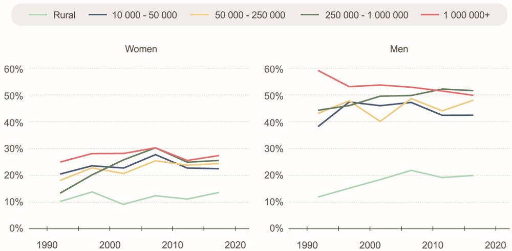
Note: Time trends have been constructed by demeaning city-level estimates from individual DHS surveys with the respective country-average across all DHS surveys, to account for the fact that the set of countries surveyed by the DHS varies from year to year. To obtain meaningful values on the vertical axis, the average across DHS surveys from all countries and years has been added. Finally, annual averages for city-size classes have been averaged into five-year bins (1990-94, 1995-99, 2000-04, 2005-09, 2010-14, 2015-19) to reduce noise. Occupational categories provided by DHS have been classified into skilled/unskilled as follows: skilled occupations are defined as professional, technical, managerial, clerical and skilled manual work. Unskilled occupations are defined as sales, agriculture, household and domestic work, services, and unskilled manual work.
Source: OECD/SWAC calculations based on ICF (1990-2019[1]) and OECD/SWAC (2018[2]).
Moreover, other data sources also point towards an absence of a significant modernisation of urban economies. Firm-level data shows that between 2010 and 2020, the share of firms engaging in R&D has declined by more than 10 percentage points. Over the same time, the share of firms engaged in export activity has remained approximately constant, even though the share of firms that follow international quality norms has declined by 5 percentage points.
Likewise, there is no indication of growing disparities in wealth or income that could be expected in a scenario in which cities lead an economic transformation. Emerging economies often experience a rise in income inequality as income levels rise, which starts to decline again as countries approach high-income status (following the well-known Kuznets curve). Rising inequality in emerging economies usually has a strong spatial dimension, as income levels in cities pull away from income levels in rural areas (see, for example, Yang (1999[26])). Yet, in Africa, no evidence of such a pattern exists. Changes in the wealth distribution have been minor.
Mirroring this trend, ownership rates of durable consumption goods have been largely stable in the past 30 years, in both cities and rural areas. For example, there has been virtually no change in average car ownership rates across cities of different sizes and rural areas (Figure 1.24).12 The share of households owning a refrigerator has grown by approximately 10 percentage points in cities as well as in rural areas, but remains below 50% even in large cities. Only the share of households owning a television has grown substantially, by 20 to 30 percentage points. This growth has been a national trend that affected cities and rural areas equally.
Figure 1.24. Evolution of car-ownership and wealth distribution by city size
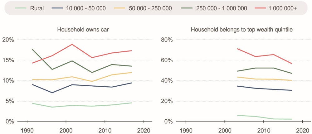
Note: Time trends have been constructed by de-meaning city-level estimates from individual DHS surveys with the respective country-average across all DHS surveys, to take into account that the set of countries surveyed by the DHS varies from year to year. To obtain meaningful values on the vertical axis, the average across DHS surveys from all countries and years has been added. Finally, annual averages for city-size classes have been averaged into five-year bins (1990-94, 1995-99, 2000-04, 2005-09, 2010-14, 2015-19) to reduce noise.
Source: OECD/SWAC calculations based on ICF (1990-2019[1]) and OECD/SWAC (2018[2]).
These trends suggest a nuanced conclusion. On the one hand, they clearly show the massive benefits of urbanisation in Africa, which are likely to continue. On the other hand, the absence of significant change in the urban economic structure indicates a persistent challenge for broader transformation. To ensure that cities drive lasting economic development, further policy measures are needed, as will be discussed in the subsequent chapters of this report.
Rural areas benefit from proximity to cities
Cities are essential for the functioning of rural economies. Depending on their size and proximity, different cities play different functions for rural areas. Cities serve as entry points to more connected and diversified economies for rural areas. They provide markets where agricultural producers can sell their products and rural households can access services and purchase basic necessities.13 In recent decades, the centre of gravity of the continent’s food system has shifted from rural areas to cities and towns. Today, cities and towns not only offer the greatest commercial opportunities for a region’s agricultural producers, but also act as nodes for food trade and markets. They are transport hubs that provide access to transport networks for goods and people. Intellectual and financial service providers, such as banks, accountants, lawyers and engineers, tend to be located in cities. Although rural businesses might need such services only infrequently, they are nevertheless indispensable for running a modern business. Often, they can be found in midsized cities, such as regional capitals, which can serve a large surrounding rural area.
Large cities offer specialised functions useful for some rural businesses. They serve as gateways to foreign markets, as they often host the local seats of multinational companies. They are usually the national financial centre, with major airports and ports. Usually, a country’s largest city is its capital and provides access to the government, which can be helpful for obtaining public tenders and influencing legislation. Large cities also tend to have the most specialised suppliers and to offer large markets of potential customers.
Being located close to cities facilitates businesses’ access to the facilities, services and market opportunities noted earlier. This reduces operating costs and offers opportunities for business development. Rural areas located close to cities can more easily be served by essential infrastructure that requires connections to larger networks, such as transport and electricity. These advantages are reflected in the structure of the economy in rural areas, which in turn influences the living standards of rural residents.
Small and medium-sized cities serve as urban hubs for rural areas
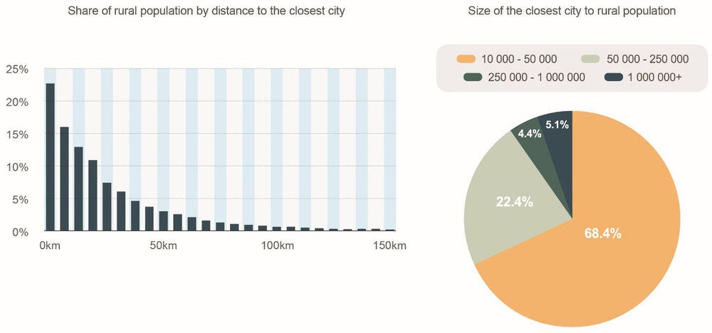
Africa’s rapid urbanisation is not only changing the urban landscape but also has profound effects on rural areas. Between 1990 and 2015, the number of cities in Africa more than doubled, from 3 319 to 7 721, with many cities emerging in rural areas with high population densities. As a direct result of the growing number of cities, more and more rural households live close to cities. Of rural residents, 50% live within 14 kilometres of a city, and 90% live within 47 kilometres. Fewer than 1.5% of rural residents are more than 100 kilometres from the closest city. Figure 1.25 shows the share of the rural population by distance to the closest city. The increasing proximity to urban areas allows a growing share of rural residents to access the services and amenities that cities offer.
Most rural households live closest to small and midsized cities. For more than two-thirds of rural residents, the closest city has between 10 000 and 50 000 inhabitants, while more than 20% of rural residents live closest to a city with between 50 000 and 250 000 inhabitants (Figure 1.25, right). In contrast, less than 10% of the rural population lives closest to a city of more than 250 000 inhabitants. These numbers underscore the importance of small and midsized cities, which are home to more than 250 million Africans (44% of the total urban population). They are also the closest urban centre for a large majority of rural households.
Figure 1.25. Distance and size of closest city to rural population
Note: Based on data for AGO, BEN, BFA, BDI, CIV, CMR, COD, COM, GAB, GHA, GIN, KEN, LBR, LSO, MDG, MLI, MOZ, MWI, NAM, NGA, RWA, SEN, SLE, TCD, TGO, TZA, UGA, ZAF, ZMB, ZWE.
Source: OECD/SWAC calculations based on ICF (1990-2019[1]) and OECD/SWAC (2018[2]).
Rural areas close to cities perform better than remote rural areas
The benefits that rural areas receive from proximity to cities become clear if outcomes are plotted against distance to the closest city. Figure 1.26 shows the share of skilled workers in rural areas depending on distance to the closest city of at least 10 000 inhabitants. In rural areas just outside cities, the share is 22%, less than half the average of the share of skilled workers in cities, but still 4 percentage points above the average for rural areas. It declines steadily with increasing distance to the closest city, up to a distance of approximately 30 kilometres, where it stabilises at approximately 13%. The share of skilled jobs in rural areas close to cities is thus almost twice as high as the share of skilled jobs in remote rural areas.
Not shown on the figure are individuals who live more than 50 kilometres away from the closest city, less than 10% of all individuals in the data. At those distances, the relationship between distance to cities and outcome variables becomes unstable and begins to fluctuate. This can partly be explained by the fact that few people live so far away from cities. The number of observations in the data is thus low, which increases the statistical noise of the estimates. However, this may partly be an indication that remote rural areas often have distinct economies, which diverge from general trends.
Figure 1.26. Share of skilled workers in rural areas by distance to nearest city
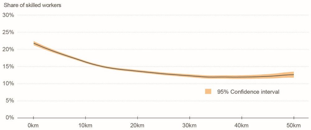
Note: Local polynomial smoothing (Epanechnikov kernel, degree = 0, bandwidth = 2.5).
Source: OECD/SWAC calculations based on ICF (1990-2019[1]) and OECD/SWAC (2018[2]).
Similar patterns can be found in a range of other outcomes. Figure 1.27 shows the relationship between distance to the closest city and outcomes such as average years of education, wealth levels, services and infrastructure access. Across all outcomes, there is a decreasing relationship with increasing distance to the nearest city, but the magnitude varies strongly from outcome to outcome. While the share of households with a bank account declines by a factor of three progressing from a distance of 1 kilometre to a distance of 50 kilometres, the relative decline in the share of residents with a mobile phone is much smaller.
Figure 1.27. Other outcomes in rural areas by distance to the closest city
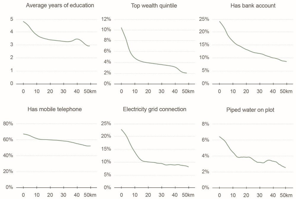
Note: Local polynomial smoothing (Epanechnikov kernel, degree = 0, bandwidth = 2.5).
Source: OECD/SWAC calculations based on ICF (1990-2019[1]) and OECD/SWAC (2018[2]).
Distance to the closest city (of any size) is by far the most important predictor of socio-economic condition. In addition, proximity to midsized cities of between 50 000 and 250 000 inhabitants, as well as proximity to large cities of above 1 million inhabitants, is correlated with better outcomes even when controlling for distance to the nearest cities. The benefits of distance to cities of different sizes are thus cumulative. When comparing two rural residents who live at a distance of 20 kilometres from a small city, but at 100 kilometres and 200 kilometres, respectively, to a large city of 1 million inhabitants, the resident closer to the large city is likely to be better off than the resident who lives farther away.
Significantly, the benefits of proximity to cities accrue regardless of the population density of rural areas. Although denser rural areas perform better in some dimensions, and rural areas that are close to cities tend to be more densely populated than remote rural areas, the benefits of proximity to cities persist even when controlling for population density in rural areas. This suggests that cities offer distinct benefits that do not emerge when the same number of people live close together in a rural setting (Annex Table 1.A.5 and Annex Table 1.A.6).
Smaller cities close to large cities perform better in some dimensions
It is not only rural areas that benefit from proximity to cities. Small and midsized cities close to large cities also perform better than small and midsized cities far from large cities, even though statistically significant correlations can be found in fewer outcomes. Notably, average years of education are higher in small and midsized cities close to large cities, which is driven in particular by a higher share of residents with secondary or higher education. This could indicate that small and midsized cities benefit from better access to education offered in large cities nearby. By contrast, the performance of small cities does not depend on whether they are located close to midsized cities. Only proximity to large cities of above 1 million inhabitants is systematically correlated with better outcomes (Annex Table 1.A.6).
References
[13] Bustos, P. (2011), “Trade Liberalization, Exports, and Technology Upgrading: Evidence on the Impact of MERCOSUR on Argentinian Firms”, American Economic Review, Vol. 101/1, pp. 304-340, https://doi.org/10.1257/aer.101.1.304.
[24] Combes, P., G. Duranton and L. Gobillon (2010), “The identification of agglomeration economies”, Journal of Economic Geography, Vol. 11/2, pp. 253-266, https://doi.org/10.1093/jeg/lbq038.
[25] Combes, P., G. Duranton and L. Gobillon (2008), “Spatial wage disparities: Sorting matters!”, Journal of Urban Economics, Vol. 63/2, pp. 723-742, https://doi.org/10.1016/j.jue.2007.04.004.
[19] Combes, P. and L. Gobillon (2015), “The Empirics of Agglomeration Economies”, in Handbook of Regional and Urban Economics, Vol. 5, pp.247-348, Elsevier, https://doi.org/10.1016/b978-0-444-59517-1.00005-2.
[15] Danert, K. and A. Healy (2021), “Monitoring Groundwater Use as a Domestic Water Source by Urban Households: Analysis of Data from Lagos State, Nigeria and Sub-Saharan Africa with Implications for Policy and Practice”, Water, Vol. 13/4, p. 568, https://doi.org/10.3390/w13040568.
[5] Gollin, D., M. Kirchberger and D. Lagakos (2021), “Do urban wage premia reflect lower amenities? Evidence from Africa”, Journal of Urban Economics, Vol. 121, p. 103301, https://doi.org/10.1016/j.jue.2020.103301.
[20] Grover, A., S. Lall and J. Timmis (2021), Agglomeration Economies in Developing Countries: A Meta-Analysis, The World Bank, https://doi.org/10.1596/1813-9450-9730.
[3] Henderson, J., D. Nigmatulina and S. Kriticos (2019), “Measuring urban economic density”, Journal of Urban Economics, p. 103188, https://doi.org/10.1016/j.jue.2019.103188.
[1] ICF (1990-2019), Demographic and Health Surveys (various datasets), https://dhsprogram.com/.
[8] ILO (2021), “ILOSTAT Explorer”, Working hours lost due to COVID-19 crisis – ILO modelled estimates (%) annual.
[23] Jacobs, J. (1969), The Economy of Cities, Random House. New York.
[14] Marin, A. et al. (2020), “Cities, Productivity, and Trade”, Working Paper No. 28309, National Bureau of Economic Research, Cambridge, Massachusetts, https://doi.org/10.3386/w28309.
[21] Marshall, A. (1890), Principles of Economics, MacMillan, London.
[16] NPC and ICF (2019), Nigeria Demographic and Health Survey 2018, National Population Commission and ICF, Abuja, Nigeria, and Rockville, Maryland.
[12] OECD (2021), Education at a Glance: OECD Indicators, OECD Publishing, Paris, https://doi.org/10.1787/19991487.
[27] OECD (2021), “Water Governance in African Cities”, OECD Studies on Water, OECD Publishing, Paris, https://dx.doi.org/10.1787/19effb77-en.
[18] OECD (2015), The Metropolitan Century: Understanding Urbanisation and its Consequences, OECD Publishing, Paris, https://dx.doi.org/10.1787/9789264228733-en.
[4] OECD/European Commission (2020), “Cities in the World: A New Perspective on Urbanisation”, OECD Urban Studies, OECD Publishing, Paris, https://dx.doi.org/10.1787/d0efcbda-en.
[2] OECD/SWAC (2018), Africapolis (database), OECD and Sahel and West Africa Club, OECD Publishing, Paris, https://africapolis.org/.
[22] Puga, D. (2010), “The magnitude and causes of agglomeration economies”, Journal of Regional Science, Vol. 50/1, pp. 203-219, https://doi.org/10.1111/j.1467-9787.2009.00657.x.
[17] UN-DESA (2019), Population Prospects, United Nations, Department of Economic and Social Affairs, Population Division, https://population.un.org/wpp/.
[10] UN-Habitat, UNECA, UNCDF and UCLGA (2020), COVID-19 in African Cities: Impacts, Responses and Policies, https://unhabitat.org/covid-19-in-africa-cities-impacts-responses-and-policies.
[9] World Bank (2021), “Responding to a stark rise in food insecurity across the poorest countries”, https://blogs.worldbank.org/voices/responding-stark-rise-food-insecurity-across-poorest-countries.
[7] World Bank (2010-2019), Enterprise Surveys, http://www.enterprisesurveys.org.
[6] World Bank (2008-2019), Living Standard Measurement Surveys, Washington DC.
[26] Yang, D. (1999), “Urban-biased policies and rising income inequality in China”, American Economic Review, Vol. 89/2, pp. 306-310, https://doi.org/10.1257/aer.89.2.306.
Annex 1.A. Tables
Annex Table 1.A.1. Main data sources used in this report
|
Country |
Available data sources |
Income group |
Level of urbanisation |
Number of cities |
Cities with available DHS data |
Cities with available LSMS data |
|---|---|---|---|---|---|---|
|
Angola |
DHS |
Lower-middle income |
63% |
96 |
75 |
0 |
|
Benin |
DHS |
Lower-middle income |
49% |
122 |
74 |
0 |
|
Burkina Faso |
DHS |
Low income |
29% |
101 |
49 |
0 |
|
Burundi |
DHS |
Low income |
21% |
33 |
20 |
0 |
|
Cameroon |
DHS |
Lower-middle income |
58% |
147 |
87 |
0 |
|
Chad |
DHS |
Low income |
29% |
93 |
46 |
0 |
|
Comoros |
DHS |
Lower-middle income |
48% |
15 |
10 |
0 |
|
Cote d’Ivoire |
DHS |
Lower-middle income |
49% |
220 |
60 |
0 |
|
Democratic Republic of the Congo |
DHS |
Low income |
45% |
553 |
85 |
0 |
|
Egypt |
DHS |
Lower-middle income |
93% |
1061 |
125 |
0 |
|
Ethiopia |
DHS/LSMS |
Low income |
27% |
510 |
97 |
299 |
|
Gabon |
DHS |
Upper-middle income |
81% |
14 |
14 |
0 |
|
Ghana |
DHS |
Lower-middle income |
52% |
209 |
121 |
0 |
|
Guinea |
DHS |
Low income |
37% |
42 |
29 |
0 |
|
Kenya |
DHS |
Lower-middle income |
65% |
126 |
95 |
0 |
|
Lesotho |
DHS |
Lower-middle income |
26% |
10 |
0 |
0 |
|
Liberia |
DHS |
Low income |
42% |
21 |
10 |
0 |
|
Madagascar |
DHS |
Low income |
22% |
68 |
21 |
0 |
|
Malawi |
DHS/LSMS |
Low income |
30% |
77 |
40 |
0 |
|
Mali |
DHS/LSMS |
Low income |
32% |
94 |
40 |
65 |
|
Mozambique |
DHS |
Low income |
33% |
167 |
37 |
16 |
|
Namibia |
DHS |
Upper-middle income |
40% |
17 |
0 |
0 |
|
Nigeria |
DHS/LSMS |
Lower-middle income |
53% |
1 236 |
76 |
0 |
|
Rwanda |
DHS |
Low income |
56% |
41 |
17 |
0 |
|
Senegal |
DHS |
Lower-middle income |
51% |
74 |
362 |
172 |
|
Sierra Leone |
DHS |
Low income |
37% |
25 |
19 |
0 |
|
South Africa |
DHS |
Upper-middle income |
70% |
502 |
62 |
0 |
|
Tanzania |
DHS/LSMS |
Lower-middle income |
38% |
249 |
25 |
0 |
|
Togo |
DHS |
Low income |
50% |
53 |
213 |
0 |
|
Uganda |
DHS/LSMS |
Low income |
39% |
125 |
149 |
148 |
|
Zambia |
DHS |
Lower-middle income |
44% |
80 |
28 |
0 |
|
Zimbabwe |
DHS |
Lower-middle income |
34% |
53 |
79 |
75 |
Note: This table lists the countries for which microdata has been available for any time between 2010 and 2019. The majority of tables and figures in this chapter are based on data from these countries. Additional and/or different datasets have been used as indicated in the notes to each table/figure.
Annex Table 1.A.2. City-size – skilled-worker-share – elasticity by country
|
|
Share of skilled worker |
|---|---|
|
|
|
|
log(pop) × AGO |
0.0444** |
|
|
(0.0166) |
|
|
|
|
log(pop) × BDI |
0.0170 |
|
|
(0.0419) |
|
|
|
|
log(pop) × BEN |
0.0356* |
|
|
(0.0156) |
|
|
|
|
log(pop) × BFA |
0.0728* |
|
|
(0.0305) |
|
|
|
|
log(pop) × CIV |
0.0138 |
|
|
(0.0253) |
|
|
|
|
log(pop) × CMR |
0.0343 |
|
|
(0.0183) |
|
|
|
|
log(pop) × COD |
0.0384* |
|
|
(0.0156) |
|
|
|
|
log(pop) × COM |
0.00487 |
|
|
(0.0910) |
|
|
|
|
log(pop) × ETH |
0.0270* |
|
|
(0.0137) |
|
|
|
|
log(pop) × GAB |
-0.00331 |
|
|
(0.0448) |
|
|
|
|
log(pop) × GHA |
0.0371 |
|
|
(0.0191) |
|
|
|
|
log(pop) × GIN |
0.0404 |
|
|
(0.0339) |
|
|
|
|
log(pop) × KEN |
0.00468 |
|
|
(0.0110) |
|
|
|
|
log(pop) × LBR |
0.0395 |
|
|
(0.0434) |
|
|
|
|
log(pop) × LSO |
0.0388 |
|
|
(0.0725) |
|
|
|
|
log(pop) × MLI |
0.00855 |
|
|
(0.0305) |
|
|
|
|
log(pop) × MOZ |
0.0414 |
|
|
(0.0222) |
|
|
|
|
log(pop) × MWI |
0.0354 |
|
|
(0.0314) |
|
|
|
|
log(pop) × NAM |
0.0721*** |
|
|
(0.0204) |
|
|
|
|
log(pop) × NGA |
0.0361*** |
|
|
(0.00794) |
|
|
|
|
log(pop) × RWA |
0.0366 |
|
|
(0.0208) |
|
|
|
|
log(pop) × SEN |
0.0477* |
|
|
(0.0210) |
|
|
|
|
log(pop) × SLE |
-0.00286 |
|
|
(0.0315) |
|
|
|
|
log(pop) × TCD |
0.0528 |
|
|
(0.0342) |
|
|
|
|
log(pop) × TGO |
0.0384 |
|
|
(0.0367) |
|
|
|
|
log(pop) × TZA |
0.00886 |
|
|
(0.0120) |
|
|
|
|
log(pop) × UGA |
0.0265 |
|
|
(0.0202) |
|
|
|
|
log(pop) × ZAF |
-0.00256 |
|
|
(0.0121) |
|
|
|
|
log(pop) × ZMB |
0.0160 |
|
|
(0.0158) |
|
|
|
|
log(pop) × ZWE |
0.0179 |
|
|
(0.0284) |
|
|
|
|
Country-year fixed effects |
YES |
|
Constant |
0.135** |
|
|
(0.0427) |
|
|
|
|
N |
2 349 |
Annex Table 1.A.3. Change over time by city-size class 2000-2020
|
|
(1) |
(2) |
(3) |
(4) |
(5) |
(6) |
(7) |
|---|---|---|---|---|---|---|---|
|
|
Years of schooling |
Share of skilled workers |
Employment share |
Share of households in top wealth quintile |
Share of households with bank account |
Electricity access |
Piped water on plot |
|
|
|
|
|
|
|
|
|
|
Linear time trend |
0.0672*** |
-0.000127 |
0.0116*** |
0.00195 |
0.00938* |
0.0102* |
0.00598 |
|
|
(0.0115) |
(0.00253) |
(0.00323) |
(0.00208) |
(0.00407) |
(0.00406) |
(0.00347) |
|
|
|
|
|
|
|
|
|
|
City 10k-50k |
1.688*** |
0.262*** |
0.0737 |
-0.220*** |
0.0112 |
0.309*** |
0.328*** |
|
|
(0.238) |
(0.0549) |
(0.0663) |
(0.0484) |
(0.0989) |
(0.0876) |
(0.0863) |
|
|
|
|
|
|
|
|
|
|
City 50k-250k |
1.993*** |
0.236*** |
0.0194 |
-0.229*** |
0.0709 |
0.405*** |
0.390*** |
|
|
(0.308) |
(0.0538) |
(0.0810) |
(0.0476) |
(0.120) |
(0.113) |
(0.0833) |
|
|
|
|
|
|
|
|
|
|
City 250k-1m |
2.094*** |
0.359*** |
0.0347 |
-0.240*** |
0.0315 |
0.366* |
0.475*** |
|
|
(0.436) |
(0.0779) |
(0.134) |
(0.0421) |
(0.154) |
(0.140) |
(0.107) |
|
|
|
|
|
|
|
|
|
|
City 1m+ |
3.141*** |
0.425*** |
-0.00295 |
-0.258*** |
0.163 |
0.583*** |
0.514*** |
|
|
(0.402) |
(0.0641) |
(0.0823) |
(0.0410) |
(0.111) |
(0.146) |
(0.0891) |
|
|
|
|
|
|
|
|
|
|
(City 10k-50k)×Year |
0.00539 |
-0.000728 |
-0.00597* |
-0.00124 |
0.00916* |
0.00212 |
-0.00424 |
|
|
(0.0112) |
(0.00273) |
(0.00286) |
(0.00220) |
(0.00415) |
(0.00388) |
(0.00370) |
|
|
|
|
|
|
|
|
|
|
(City 50k-250k)×Year |
0.0199 |
0.00215 |
-0.00417 |
-0.00224 |
0.00957 |
0.00124 |
-0.00391 |
|
|
(0.0158) |
(0.00260) |
(0.00356) |
(0.00210) |
(0.00493) |
(0.00527) |
(0.00371) |
|
|
|
|
|
|
|
|
|
|
(City 250k-1m)×Year |
0.0231 |
-0.000905 |
-0.00512 |
-0.00297 |
0.0115 |
0.00542 |
-0.00612 |
|
|
(0.0214) |
(0.00343) |
(0.00574) |
(0.00202) |
(0.00664) |
(0.00618) |
(0.00476) |
|
|
|
|
|
|
|
|
|
|
(City 1m+)×Year |
0.00453 |
-0.00434 |
-0.00159 |
-0.00192 |
0.00824 |
-0.00106 |
-0.00605 |
|
|
(0.0183) |
(0.00334) |
(0.00407) |
(0.00193) |
(0.00468) |
(0.00693) |
(0.00422) |
|
|
|
|
|
|
|
|
|
|
Country fixed effects |
YES |
YES |
YES |
YES |
YES |
YES |
YES |
|
Constant |
1.552*** |
0.195*** |
0.529*** |
0.271*** |
-0.0556 |
0.0540 |
-0.0529 |
|
|
(0.246) |
(0.0514) |
(0.0751) |
(0.0462) |
(0.0984) |
(0.0895) |
(0.0814) |
|
|
|
|
|
|
|
|
|
|
N |
3 350 |
2 833 |
2 853 |
3 803 |
2 884 |
3 937 |
3 937 |
Note: All dependent variables are averages at the city level, as available from DHS surveys between 2000 and 2020. Cities 10k-50 – Cities 1m+ are a set of dummy variables indicating whether the city fell into the corresponding size class in 2000. Rural areas are the omitted base category. Standard errors cluster at country-year level in parentheses, * p<0.05, ** p<0.01, *** p<0.001. Specifications (2) and (3) use averages for male respondents only.
Annex Table 1.A.4. Evolution of the occupation share by city-size class over time
|
|
(1) |
(2) |
(3) |
(4) |
(5) |
(6) |
(7) |
(8) |
|---|---|---|---|---|---|---|---|---|
|
|
Professional/ technical/ managerial |
Clerical |
Sales |
Agriculture |
Household and domestic |
Services |
Skilled manual |
Unskilled manual |
|
|
|
|
|
|
|
|
|
|
|
Linear time trend |
0.00206* |
0.000786* |
0.00190 |
-0.000240 |
0.000570 |
0.00219* |
0.00116 |
0.00303* |
|
|
(0.000844) |
(0.000299) |
(0.00143) |
(0.00460) |
(0.000536) |
(0.00102) |
(0.00139) |
(0.00117) |
|
|
|
|
|
|
|
|
|
|
|
City 10k-50k |
0.0776*** |
0.0164*** |
0.0412* |
-0.322*** |
0.00812 |
0.0315** |
0.101*** |
0.0357** |
|
|
(0.0120) |
(0.00458) |
(0.0181) |
(0.0481) |
(0.00442) |
(0.0116) |
(0.0173) |
(0.0105) |
|
|
|
|
|
|
|
|
|
|
|
City 50k-250k |
0.0642*** |
0.00919 |
0.0619*** |
-0.395*** |
0.00437 |
0.0491* |
0.117*** |
0.0585*** |
|
|
(0.0165) |
(0.00765) |
(0.0160) |
(0.0566) |
(0.00609) |
(0.0204) |
(0.0194) |
(0.0147) |
|
|
|
|
|
|
|
|
|
|
|
City 250k-1m |
0.0515*** |
0.0162* |
0.0660** |
-0.479*** |
0.00719 |
0.0556* |
0.172*** |
0.0477* |
|
|
(0.0145) |
(0.00698) |
(0.0229) |
(0.0648) |
(0.0120) |
(0.0271) |
(0.0482) |
(0.0184) |
|
|
|
|
|
|
|
|
|
|
|
City 1m+ |
0.0975*** |
0.0261*** |
0.101*** |
-0.517*** |
0.00487 |
0.0443* |
0.165*** |
0.0525** |
|
|
(0.0152) |
(0.00635) |
(0.0218) |
(0.0577) |
(0.00613) |
(0.0191) |
(0.0244) |
(0.0192) |
|
|
|
|
|
|
|
|
|
|
|
(City 10k-50k)×Year |
-0.000205 |
-0.000312 |
0.00109 |
-0.00428 |
0.0000204 |
0.00139 |
-0.000743 |
-0.00175* |
|
|
(0.000997) |
(0.000344) |
(0.00149) |
(0.00409) |
(0.000344) |
(0.000918) |
(0.00142) |
(0.000828) |
|
|
|
|
|
|
|
|
|
|
|
(City 50k-250k)×Year |
0.000857 |
0.000636 |
-0.000896 |
-0.00302 |
0.000505 |
0.000986 |
-0.000595 |
-0.00249 |
|
|
(0.00152) |
(0.000715) |
(0.00137) |
(0.00493) |
(0.000528) |
(0.00155) |
(0.00159) |
(0.00129) |
|
|
|
|
|
|
|
|
|
|
|
(City 250k-1m)×Year |
0.00288* |
-0.000120 |
-0.000834 |
-0.000504 |
0.000670 |
0.000658 |
-0.00264 |
-0.00199 |
|
|
(0.00141) |
(0.000521) |
(0.00174) |
(0.00575) |
(0.00105) |
(0.00214) |
(0.00351) |
(0.00146) |
|
|
|
|
|
|
|
|
|
|
|
(City 1m+)×Year |
0.000164 |
-0.000232 |
-0.00245 |
0.00173 |
0.000673 |
0.00239 |
-0.00217 |
-0.00156 |
|
|
(0.00120) |
(0.000487) |
(0.00174) |
(0.00563) |
(0.000554) |
(0.00141) |
(0.00208) |
(0.00154) |
|
Country fixed effects |
YES |
YES |
YES |
YES |
YES |
YES |
YES |
YES |
|
|
|
|
|
|
|
|
|
|
|
Constant |
0.0168 |
-0.00287 |
0.0305 |
0.541*** |
-0.00180 |
0.00445 |
0.0764*** |
0.0138 |
|
(0.00996) |
(0.00351) |
(0.0171) |
(0.0511) |
(0.00723) |
(0.0137) |
(0.0165) |
(0.0127) |
|
|
|
|
|
|
|
|
|
|
|
|
N |
2 851 |
2 851 |
2 851 |
2 851 |
2 851 |
2 851 |
2 851 |
2 851 |
Note: All dependent variables are averages at the city level, as available from DHS surveys between 2000 and 2020. Cities 10k-50k – Cities 1m+ are a set of dummy variables indicating whether the city fell into the corresponding size class in 2000. Rural areas are the omitted base category. Standard errors cluster at country-year level in parentheses, * p<0.05, ** p<0.01, *** p<0.001. Specifications (2) and (3) use averages for male respondents only.
Annex Table 1.A.5. Distance to closest city and outcomes in rural areas
|
|
(1) |
(2) |
(3) |
(4) |
(5) |
(6) |
(7) |
(8) |
(9) |
(10) |
(11) |
(12) |
|---|---|---|---|---|---|---|---|---|---|---|---|---|
|
|
Log (years of education) |
Log (years of education) |
Has bank account |
Has bank account |
Has mobile phone |
Has mobile phone |
Electricity grid connection |
Electricity grid connection |
Piped water on plot |
Piped water on plot |
Top wealth quintile |
Top wealth quintile |
|
Log distance to closest city |
-0.0571** |
-0.0522* |
-0.0113*** |
-0.0105*** |
-0.0193*** |
-0.0169*** |
-0.0199*** |
-0.0160*** |
-0.00874*** |
-0.00506*** |
-0.00930*** |
-0.00761*** |
|
(0.0212) |
(0.0205) |
(0.00221) |
(0.00220) |
(0.00247) |
(0.00254) |
(0.00365) |
(0.00381) |
(0.00176) |
(0.00140) |
(0.00134) |
(0.00166) |
|
|
Log distance to closest city above 50k inhabitants |
-0.139*** |
-0.112*** |
-0.00824** |
-0.00610* |
-0.0101** |
-0.00344 |
-0.00359 |
-0.000782 |
0.00320 |
0.00163 |
-0.00245 |
-0.00447** |
|
(0.0254) |
(0.0295) |
(0.00278) |
(0.00278) |
(0.00304) |
(0.00312) |
(0.00286) |
(0.00293) |
(0.00219) |
(0.00218) |
(0.00152) |
(0.00141) |
|
|
Log distance to closest city above 250k inhabitants |
0.111* |
0.116** |
0.00243 |
0.00193 |
-0.000907 |
0.000439 |
-0.00331 |
-0.00335 |
-0.00487 |
-0.00155 |
0.000574 |
0.000681 |
|
(0.0441) |
(0.0409) |
(0.00347) |
(0.00354) |
(0.00616) |
(0.00644) |
(0.00547) |
(0.00552) |
(0.00364) |
(0.00295) |
(0.00224) |
(0.00236) |
|
|
Log distance to closest city of above 1m inhabitants |
-0.173*** |
-0.176** |
-0.00638 |
-0.00491 |
-0.0152* |
-0.0149 |
-0.0107 |
-0.0105 |
-0.00329 |
-0.00366 |
-0.00675* |
-0.00893** |
|
(0.0486) |
(0.0544) |
(0.00380) |
(0.00397) |
(0.00715) |
(0.00769) |
(0.00653) |
(0.00653) |
(0.00228) |
(0.00204) |
(0.00278) |
(0.00297) |
|
|
Distance to closest port |
-0.344** |
-0.313* |
-0.0165 |
-0.0143 |
-0.0165* |
-0.00910 |
-0.0206** |
-0.0153** |
-0.000277 |
0.00365 |
-0.00507 |
-0.00378 |
|
(0.119) |
(0.129) |
(0.00977) |
(0.0101) |
(0.00724) |
(0.00769) |
(0.00625) |
(0.00551) |
(0.00216) |
(0.00232) |
(0.00382) |
(0.00450) |
|
|
Log population within 10km radius |
0.122*** |
0.00756* |
0.0228*** |
0.0322*** |
0.0140*** |
0.0122** |
||||||
|
(0.0265) |
(0.00302) |
(0.00469) |
(0.00517) |
(0.00363) |
(0.00397) |
|||||||
|
Log population within 50km radius |
-0.0373 |
-0.00267 |
-0.00144 |
-0.0146* |
-0.00479 |
-0.0120** |
||||||
|
(0.0519) |
(0.00489) |
(0.00806) |
(0.00624) |
(0.00375) |
(0.00360) |
|||||||
|
Country-year fixed effects |
YES |
YES |
YES |
YES |
YES |
YES |
YES |
YES |
YES |
YES |
YES |
YES |
|
Constant |
5.186*** |
4.086** |
0.306*** |
0.232* |
0.835*** |
0.531*** |
0.363*** |
0.172 |
0.0901*** |
-0.0330 |
0.139*** |
0.179** |
|
(0.669) |
(1.274) |
(0.0588) |
(0.104) |
(0.0402) |
(0.132) |
(0.0475) |
(0.0931) |
(0.0166) |
(0.0654) |
(0.0222) |
(0.0521) |
|
|
N |
2 140 291 |
2 140 291 |
2 525 596 |
2 525 596 |
2 614 059 |
2 614 059 |
2 613 871 |
2 613 871 |
2 614 177 |
2 614 177 |
2 615 091 |
2615091 |
Note: The sample includes all rural individuals covered by DHS surveys in Africa between 2010 and 2019. Standard errors cluster at country-year level in parentheses, * p<0.05, ** p<0.01, *** p<0.001.
Annex Table 1.A.6. Distance to city of above 1 million inhabitants and outcomes in cities
|
(1) |
(2) |
(3) |
(4) |
(5) |
(6) |
(7) |
|
|---|---|---|---|---|---|---|---|
|
Log years of schooling |
Completed secondary or higher education |
Has bank account |
Top wealth quintile |
Has electricity |
Piped water on plot |
Has mobile phone |
|
|
Log population |
0.0499** |
0.0284*** |
0.0354*** |
0.0646*** |
0.0542*** |
0.0272*** |
0.0211*** |
|
(0.0185) |
(0.00699) |
(0.00758) |
(0.0128) |
(0.0104) |
(0.00675) |
(0.00531) |
|
|
Log distance to closest city with 1 million inhabitants |
-0.0564** |
-0.0242** |
-0.0145 |
-0.0312** |
-0.0163 |
-0.0189* |
-0.0107 |
|
(0.0178) |
(0.00832) |
(0.00803) |
(0.00940) |
(0.0126) |
(0.00905) |
(0.00674) |
|
|
Log population within 10km |
0.0443 |
0.0166 |
0.0122 |
0.0186 |
0.00465 |
0.0435*** |
0.0120 |
|
(0.0274) |
(0.00883) |
(0.00842) |
(0.0125) |
(0.0119) |
(0.0117) |
(0.00752) |
|
|
Log population within 50km |
0.00396 |
-0.00633 |
0.00233 |
-0.00448 |
-0.00697 |
-0.0346* |
-0.00442 |
|
(0.0234) |
(0.00932) |
(0.00863) |
(0.0127) |
(0.0144) |
(0.0161) |
(0.00640) |
|
|
Country-year fixed effects |
YES |
YES |
YES |
YES |
YES |
YES |
YES |
|
Constant |
1.064** |
0.223 |
-0.0554 |
-0.345 |
0.167 |
0.0555 |
0.620*** |
|
(0.352) |
(0.134) |
(0.116) |
(0.214) |
(0.203) |
(0.159) |
(0.151) |
|
|
N |
2 440 |
2 441 |
2 737 |
3 022 |
3 022 |
3 022 |
3 022 |
Annex Table 1.A.7. City-size elasticity of wages
|
Log hourly wage |
||||
|---|---|---|---|---|
|
|
(1) |
(2) |
(3) |
(4) |
|
|
||||
|
Log city-population |
0.025* |
0.030** |
0.124*** |
0.121*** |
|
|
(0.013) |
(0.013) |
(0.025) |
(0.029) |
|
|
||||
|
Log area |
-0.108*** |
-0.098*** |
||
|
|
(0.024) |
(0.027) |
||
|
|
||||
|
Observations |
10 127 |
8 919 |
10 127 |
8 919 |
|
Adjusted R-squared |
0.810 |
0.819 |
0.811 |
0.819 |
|
Country-year fixed effects |
X |
X |
X |
X |
|
Individual controls |
X |
X |
X |
X |
|
Geographical controls |
X |
X |
||
|
N |
8 919 |
8 919 |
8 919 |
8 919 |
Note: Individual controls include age, age-squared, gender, education, household size, hours worked and occupation. Geographical controls include dummies for vegetation zones and distance to the closest city of above 1 million inhabitants. Standard errors are clusters at the city level. Urban residents only.
Annex Table 1.A.8. Wage differentials by city-size class
|
|
Log hourly wage |
|---|---|
|
|
|
|
City with 10k-50k inhabitants |
0.209*** |
|
|
(0.050) |
|
|
|
|
City with 50k-250k inhabitants |
0.191*** |
|
|
(0.047) |
|
|
|
|
City with 250k-1m inhabitants |
0.147*** |
|
|
(0.050) |
|
|
|
|
City with 1 million+ inhabitants |
0.287*** |
|
|
(0.076) |
|
|
|
|
Observations |
16 359 |
|
Adjusted R-squared |
0.786 |
|
Country X-Year fixed effects |
X |
|
Individual controls |
X |
|
Geographical controls |
X |
|
N |
16 359 |
Note: Individual controls include age, age-squared, gender, education, household size, hours worked and occupation. Geographical controls include dummies for vegetation zones and distance to the closest city above 1 million inhabitants. Rural inhabitants are the baseline category.
Notes
← 1. It should be noted that wage and consumption data is calculated from Living Standard Measurement Survey data, which contains observations from only 30 000 individuals in six countries. The estimates are thus much less precise than the majority of the estimates in this chapter, which are based on more than 4 million observations collected by the Demographic and Health Survey from 32 countries.
← 2. This probability has been calculated by matching the built-up areas defined by Africapolis with the spatial population distribution according to the WorldPop population grid (Linard et al., 2012[28]; WorldPop[29]).
← 3. This statistic is based on a DHS wealth index classification of households into wealth quintiles. As some scholars criticise the DHS wealth index for underestimating the wealth of rural households, the figures potentially underestimate wealth levels in rural areas in comparison to urban areas.
← 4. See OECD (2021[27]) for a discussion of the governance challenges involved in providing water infrastructure.
← 5. Labour productivity is proxied by wages, as is common in the literature on the topic.
← 6. Per capita GDP in cities is predicted to increase by 0.22 percentage points. Because almost exactly half of Africa’s population lives in cities, this contributes 0.11 percentage points to overall per capita GDP growth.
← 7. Averages from 2000-2010 are used because they are more reliable than data for later periods. In the absence of censuses, recent population data is often based on projections and tends underestimate urbanisation.
← 8. This assumption implies that total factor productivity (TFP) growth due to agglomeration economies is identical to labour productivity growth and that the employment rate and capital stock remain unaffected by urbanisation.
← 9. In the early 1990s, 62% of the 190 million urban residents were connected to the electricity grid, but by the late 2010s, the share had risen to 72% of the 700 million urban residents.
← 10. In the early 2000s, 23% of the 290 million urban residents lived in households with bank accounts, while in the late 2010s, the share had risen to 48% of the 700 million urban residents.
← 11. Although it might appear that there are differential trends for the share of male skilled workers in cities of between 250 000 and 1 million inhabitants and cities of more than 1 million, Annex Table 1.A.4 shows that these trends are not significant (i.e. they are statistically indistinguishable from chance).
← 12. This does not conflict with the fact that car ownership levels at the national level have risen, as people moved from rural areas with low car ownership rates to cities with higher car ownership rates.
← 13. As countries develop, the importance of market towns as points of sale for agricultural producers declines, because of the emergence of wholesale traders that reduce the reliance on local markets. At the same time, market towns become more important as places to purchase goods, as living standards and disposable incomes of rural populations rise.
