This chapter undertakes a diagnosis of productivity and innovation levels in the United States, by comparing metropolitan and non-metropolitan counties with predominantly urban or rural characteristics. It identifies strengths and challenges for innovation in rural areas, and sets the scene for the policy discussions of the report. It pays special regard to geographic disparities and to equal opportunities for education, entrepreneurship and innovation in rural counties.
Enhancing Rural Innovation in the United States

2. Understanding innovation in rural United States
Abstract
Key messages
There is convergence in productivity between counties, bringing urban and rural parts of the country closer together
There is a gap in performance of rural vis-à-vis metropolitan regions.1 In the United States, the gap between the top- and bottom-performing regions is 12% greater than the average of OECD countries. The GDP gap, which measures the difference in real GDP per capita between the richest (top 20%) and poorest (bottom 20%) regions, averaged USD 30 890 for 26 OECD countries with available regional data from 2008 to 2020. At USD 34 551, The US GDP gap was higher than 18 countries and lower than 7 others. Taking the size of GDP into account, the US gap is 62% of its GDP per capita, against an international average of 85%. Of the regions reported to be in the top 20% of GDP, 70% are in metropolitan regions (MR-L and MR-M) and 26% are in rural regions (NMR-R), against 26% and 61% for the bottom 20%, respectively.
In county level analysis, the gap in GDP per capita is declining, but in a volatile way. While contributing the smallest share of GDP of the total economy, rural counties led in GDP per capita growth in the decade between 2010 to 2020, averaging 1.5% per year against metropolitan (urban) counties’ 0.9%. At the same time, growth in completely rural counties and other non‑metropolitan counties was more volatile than growth in metropolitan counties owing to their exposure to global market conditions in sectors such as agriculture and manufacturing.
Convergence in labour productivity between counties is led by rural growth. Labour productivity in rural counties surged between 2009 and 2020, averaging 1.7% annually as it converged towards that of metropolitan counties. Likewise, non-metropolitan counties adjacent to cities caught up to non-metropolitan counties not adjacent to cities, albeit at a slower annualised rate of 0.9%. Across the decade, productivity disparity remained the highest in rural counties, having the greatest share of the most and least productive firms.
Structural change is impacting economic activity in rural areas
The face of the rural economy is changing. In 2020, as a share of the total economy, rural counties in the United States were dominated by finance and real estate (24%), agriculture (23%), and manufacturing (13%), a ranking unchanged from 2010. However, even these sectors are employing a lower share of workers in 2020 than in 2010, and 9 out of 12 sectors in rural counties shed their share of jobs across the decade. In rural counties, the top employers are in education and social services (24%), manufacturing (13%), and retail trade (11%). Thus, despite often being viewed as agrarian, manufacturing and services sectors actually employ more workers than the agriculture sector in rural counties.
Productivity growth is coinciding with a relative drop in employment in non-metropolitan counties as compared to previous years. Despite the reduction in relative labour resources, the remaining share of employment within non-metropolitan counties still leads to productivity gains. Decomposition analysis that separates the effects of more efficient use of resources (“within” effect) versus reallocation of resources across typologies of counties (“between” effect) finds that most productivity growth is primarily due to more efficient use of resources within each type of county. In fact, over the past 10 years, most of the productivity growth in non-metro counties has been primarily due to more efficient use of resources within counties, despite the negative impact of the reallocation of production factors, like labour or capital in non-metropolitan areas.
The context for innovation is different in non-metropolitan and metropolitan counties
Innovation happens through interactions between people and firms in places that are able to provide the right setting (Crescenzi, Nathan and Rodríguez-Pose, 2016[1]). At the same time, new jobs bring in a new mix of individuals who have the potential to innovate. Counties with larger shares of inventive workers also tend to have high number of employed individuals, but not necessarily equally higher labour productivity.
Places where there are high levels of firm activity (clustering) are often associated with local innovation outcomes (Delgado, Porter and Stern, 2014[2]). In non-metropolitan areas, there can be a penalty associated with this in part because of fewer interactions and interconnectedness with firms elsewhere, especially when it comes to science- and technology-based innovation.
High-tech innovation is less prevalent in rural areas. On average, individuals with inventive occupations (as described in Annex 2.C) living in non-metropolitan and rural counties have applied for fewer patents than those in metropolitan areas. There are 1.3 fewer patents per 1 000 “inventive” individuals in non-metropolitan areas, as compared to metropolitan areas, despite controlling for standard sectoral and economic factors.
On the other hand, innovation absorption, a driver of overall productivity and growth, is stronger in rural and non-metropolitan counties. For example, nearly two-thirds of overall productivity growth from 2010 to 2020 was due to innovation absorption in non-metropolitan areas.
There is more room for gains from innovation in rural and non-metropolitan counties. On average, rural and non-metropolitan counties have less patent intensity as compared to metro counties. Yet patent intensity in non-metropolitan counties is still positively correlated with R&D expenditure per worker, whereas this is not the case in metropolitan counties.
There is a margin of opportunity for innovation in non- metropolitan counties.
For every 1% increase in R&D spending, patent intensity increases by 0.7 units in non-metropolitan counties, while it is close to zero, and more spurious in metropolitan counties.
Investing in the education of the workforce is also associated with higher patent intensity and productivity in non-metropolitan regions.
Investing in education is positively associated with increases in productivity in non-metropolitan counties. A 1% increase in government spending in education (per capita) is associated with a 0.54% increase in productivity (output per worker) in non-metropolitan counties. As compared to metropolitan counties, the marginal increase to the additional percentage of government spending is lower, at 0.30%.
A 1 unit increase in the share of tertiary educated workforce is associated with 1.1 increase in patent intensity in non-metropolitan counties. However, the magnitude in non-metropolitan counties is lower than in metropolitan counties where the magnitude of the relation is at 2.1, suggesting that one may need to look beyond tertiary education for innovation in non-metropolitan counties.
Critically, for innovation in non-metropolitan areas, educational institutions need to be suitable for local communities. Higher Education and Research and Development (HERD) institutions play an unequal role across counties. While an increase in the number of HERD institutions is associated with a 1.6% increase in productivity in metropolitan regions, it does not drive productivity in non-metropolitan regions. Its effect on patent intensity is positive in metropolitan counties, but non-significant for both metropolitan and non-metropolitan counties. Evidence suggests that higher education institutions with close ties to the economy in rural counties may have a more positive impact on local innovation.
Equitable opportunities for innovation and entrepreneurship is an important factor to consider
Compared with 18 other OECD countries, overall GDP inequality in the US is above average, driven by high disparities in rural counties and non-metropolitan counties not adjacent to cities. Furthermore, inequality in the US is growing, with relatively high levels in the more remote counties.
Government support often targets places that have demographic challenges or have systematically been left behind. Indeed, the share of persistently poor2 counties is five times higher in rural counties than in metropolitan counties. Enabling equal opportunities for access to entrepreneurship and innovation should be a priority across counties, especially considering that:
The United States has an aging workforce, with non-metropolitan counties having a relatively larger share of older workforce population than metropolitan counties.
While gender inequality has lessened, on average, women in rural counties still face larger wage inequality than those in metropolitan counties.
Priority should be placed on policies aiming to deliver equitable access to services in non‑metropolitan regions to support the efforts in reducing persistent poverty within counties.
1. See Annex 2.A for further description on comparative regional classifications of metropolitan and non-metropolitan regions (including rural remote regions). See Table 2.1 and Annex 2.A for further description of classifications of counties based on the United States Department for Agriculture’s (USDA) Rural-Urban Continuum Classification.
2. The definition adopted for “persistently poor” counties is defined by congress and used by departments such as the US Department of Commerce. According to a Congressional requirement, a county (or a county-level equivalent) is experiencing Persistent Poverty if their most recent poverty rate estimate, within the margin of error, equates to 20 percent, while also evidencing poverty rates of at least 20 percent in the 1990 and 2000 decennial censuses (i.e., 20 percent or greater poverty over the last 30 years) (Consolidated Appropriations Act, 2021, P.L. 116-260 (Dec. 27, 2020), Explanatory Statement of the House Committee on Appropriations, 116 Cong. Rec. H7879, 2020, https://www.congress.gov/116/plaws/publ260/PLAW-116publ260.pdf)).
The United States is one of the global leaders in the field of innovation. Its high levels of protection for intellectual property rights, quality of higher education institutions, and levels of competition between firms lends itself to creating an environment for cutting-edge research and high-tech innovation. However, innovation is not equally distributed across areas, with high-tech innovation clustered in a few states with relatively large metropolitan populations. Geographical clustering is consistent across most OECD countries and can be a challenge for policymakers. A particular challenge is how innovation and entrepreneurship can be promoted within districts or states that have low density and are far from metropolitan centres where access to services and supply chains may be less challenging.
The United States has a strong federal mandate to promote innovation and entrepreneurship. It is a responsibility shared by several government departments including the Department of Commerce, the Department of Agriculture, the National Science Foundation, Department of Defense, Department of Energy and National Aeronautics and Space Administration.
There is no national strategy that considers innovation and entrepreneurship with a rural lens. For government officials focused on regional and rural development, larger scale projects for high-tech innovation often overlook the structure of rural and regional economies, and the characteristics of innovation across geographies. Despite that, the Economic Development Administration (EDA) of the Department of Commerce and, to a larger extent, the United States Department of Agriculture (USDA) are often tasked with understanding how to promote innovation and entrepreneurship in rural areas.
As in other federal OECD countries, co-ordination and collaboration on joint priorities between the federal and state governments can be a challenge (OECD, 2022[3]; OECD, forthcoming[4]). In addition, difficulties related to scale and state hegemony over key framework conditions such as access to finance, education and digital infrastructure, can make addressing bottlenecks for promoting innovation and entrepreneurship more complicated.
This chapter sets the scene for understanding rural and non-metropolitan counties, trends in innovation and a few drivers of innovation and equitable opportunities in non-metropolitan regions. Drawing on broad trends, it focuses on evidence and analysis in non-metropolitan counties, as well as their characteristics and capacity to innovate.
To explore trends and set the scene for the rest of the chapter, the analysis uses pooled data from the American Community Survey (ACS), the Bureau of Economic Analysis (BEA), the U.S. Decennial Census and the United States Patent and Trademark Office (USPTO). For the most part, analysis is conducted from 2000 to 2020, or the most recent year available at county level. There are usually over 3 000 observations per year, although in some cases data may be missing for some counties. County-level data is then reported on an aggregated level based on geographical classifications. The ACS provides statistics on employees and in some cases firms, but the majority of the data on firms is gathered from the BEA regional tables.
Setting the scene for rural innovation in the United States
No examination of rurality could start without an appropriate definition of “rural” and “urban”. In this report, we adopt the United States Department of Agriculture (USDA)’s classification to distinguish between rural and urban counties,1 known as the Rural-Urban Continuum Codes (RUCC). It assigns each county in the United States to nine different codes, taking into account the degree of urbanisation and adjacency to metro areas, as demonstrated in Table 2.1. The latest version of the RUCC was published in 2013 and classifies all 1 167 metropolitan counties and 1 976 non-metropolitan counties in the United States, including 69 metro municipalities and 9 non-metro municipalities in Puerto Rico and each Census Bureau-designated county-equivalent area of the Virgin Islands and other inhabited island territories of the United States (USDA, 2013[5]). The analysis in this chapter will use a simplified version of the classification as indicated in the fifth column of Table 2.1. Further description of this classification system and those used in wider OECD work are described in detail in Annex 2.A.
Table 2.1. 2013 Rural-Urban Continuum Codes
|
Code |
Description |
Number of counties |
2010 population (on which the classification is based) |
Simplified classification (used in report) |
|---|---|---|---|---|
|
Metro counties |
||||
|
1 |
Counties in metro areas of 1 million population or more |
432 |
168 523 961 |
Metropolitan (Metro) |
|
2 |
Counties in metro areas of 250 000 to 1 million population |
379 |
65 609 956 |
Metropolitan (Metro) |
|
3 |
Counties in metro areas of fewer than 250 000 population |
356 |
28 318 215 |
Metropolitan (Metro) |
|
Total |
1 167 |
262 452 132 |
||
|
Non-metro counties |
||||
|
4 |
Urban population of 20 000 or more, adjacent to a metro area |
214 |
13 538 322 |
Non-metropolitan adjacent to urban area (Non-metro AU) |
|
5 |
Urban population of 20 000 or more, not adjacent to a metro area |
92 |
4 953 810 |
Non-metropolitan non‑adjacent to urban area (Non-metro NAU) |
|
6 |
Urban population of 2 500 to 19 999, adjacent to a metro area |
593 |
14 784 976 |
Non-metropolitan adjacent to urban area (Non-metro AU) |
|
7 |
Urban population of 2 500 to 19 999, not adjacent to a metro area |
433 |
8 248 674 |
Non-metropolitan non‑adjacent to urban area (Non-metro NAU) |
|
8 |
Completely rural or less than 2 500 urban population, adjacent to a metro area |
220 |
2 157 448 |
Non-metropolitan, completely rural (Rural) |
|
9 |
Completely rural or less than 2 500 urban population, not adjacent to a metro area |
424 |
2 610 176 |
Non-metropolitan completely rural (Rural) |
|
Total |
1 976 |
46 293 406 |
||
|
US total |
3 143 |
308 745 538 |
||
Source: Based on USDA (2013[5]), Rural-Urban Continuum Codes, https://www.ers.usda.gov/data-products/rural-urban-continuum-codes.
This report approaches innovation through a framework that places a focus on the capacity for people to innovate in non-metropolitan areas. For this purpose, individuals and their characteristics feature in measurement approaches, and when this is not possible, we also include demographic characteristics of places. Approaching the measurement of innovation from a rural perspective requires understanding the structure, opportunities and strengths of rural regions and reflecting on whether commonly accepted indicators of innovation adequately reflect innovation in rural areas. One possible strategy is to use survey-based methods that define innovation in a commonly accepted way. To this day, the most commonly used definition of innovation is the Oslo definition, as described in Annex 2.B. However, no one single innovation survey exists with a large enough sample size in rural areas to make it representative for rigorous analysis, thus creating a barrier to its application to policies and programmes in rural areas.
Other measurement methods could include product-level data, research and development investment and jobs, patents, high-growth or productivity, or start-up entrepreneurship statistics that each proxy some measurement of innovation (OECD, 2022[6]). However, when using non-survey-based methods, analysis should be nuanced to avoid the exclusion of the types of innovation that are not easily measurable in rural areas, and where measurement meets policy, to focus on the capacity to innovate.
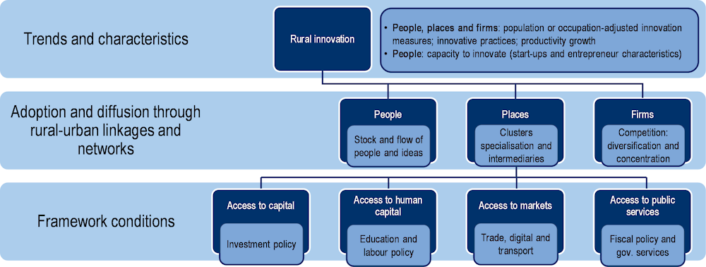
When possible, the report adjusts innovation statistics using a rural lens as described in Annex 2.B. The decision to frame this discussion was based on consultation with business and academic experts in the OECD Enhancing Rural Innovation project advisory committee. Figure 2.1 describes the proposed framework for understanding innovation within the rural context that sets the scene throughout the report. It takes a more critical view of the different forms of innovation in a rural setting, identifies the place-based framework conditions such as access to human capital, financial capital, markets and public services, as well as the critical role of linkages and networks for building scale in places with low density and large distances to urban centres.
Figure 2.1. Analytical framework for understanding the drivers of innovation in rural areas
Note: Public services include direct support mechanisms.
Source: OECD (2022[6]), Unlocking Rural Innovation, https://doi.org/10.1787/9044a961-en.
Understanding economic activities and rural well-being in the United States
The data used in this section’s analysis is sourced from the American Community Survey 5-year estimates (ACS) (2022[7]) and the Bureau of Economic Analysis’ (BEA) Regional Economic Accounts (2022[8]). Of the 3 141 counties in the United States (Table 2.1), data was available for the majority of counties and years (between 2010 and 2020), but not in all cases. For data from the BEA, where statistics on regional GDP and employment are generated, the percentage of missing data is around 3.1% for metro, 1.6% for non-metro adjacent to urban (AU), 0.8% for non-metro non-adjacent to urban (NAU), and 0% for metro. For the ACS, from which the population series is sourced, coverage is nearly 100%.
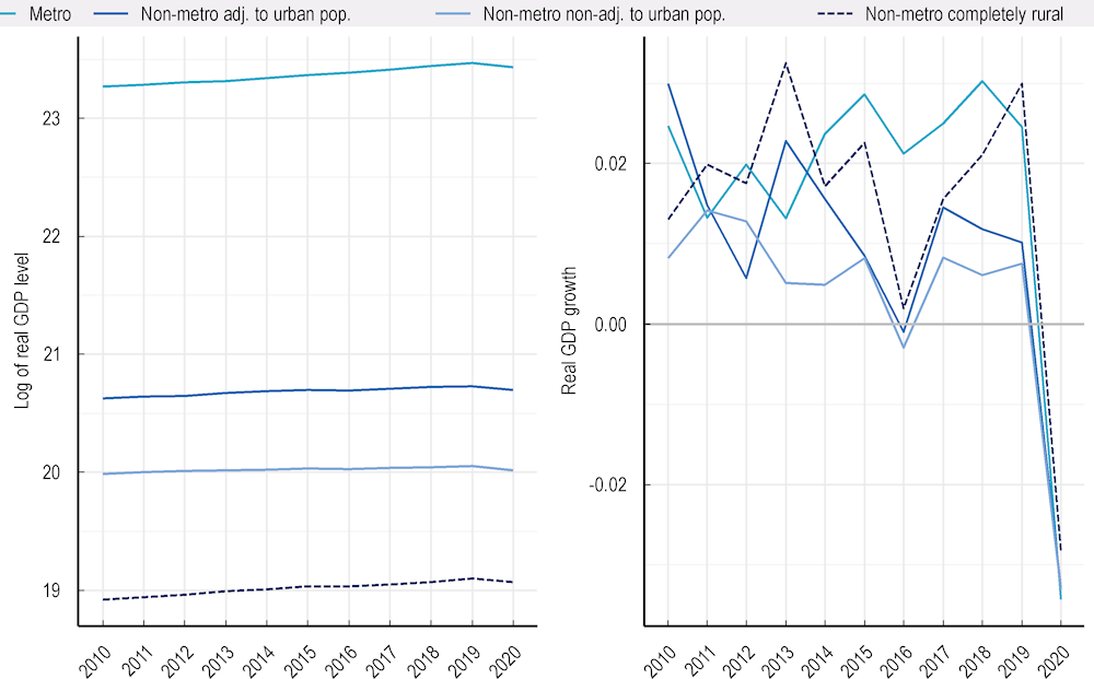
Perhaps unsurprisingly, metropolitan counties of the United States generate the lion’s share of all private economic activity and employment. Metropolitan areas, according to the simplified classification, accounted for almost 90% of the economy in 2020 (Figure 2.2, left). Of the remaining 10%, Non-metro AU contributed 5.8%, followed by Non-metro NAU (3.3 %), and Rural counties (1.2%). While the spatial distribution of non‑government GDP has remained stable when compared to 2010, we observe that increases in GDP shares took place in metro counties (0.7 percentage points) and rural counties (0.1 percentage points). Non-metro AU and non-metro NAU saw a shrinkage of 0.4 and 0.3 percentage points, respectively.
While there is a large population living in non-metropolitan areas of the United States, the share of individuals living in non-metropolitan areas is relatively small as compared to most OECD countries. In OECD countries, we observe close to 29% of individuals living in non-metropolitan and rural areas based on OECD-wide harmonised definitions (Fadic et al., 2019[9]; OECD, 2022[3]).2 In the United States, using the same definition, only 15.6% of individuals were living in non-metropolitan and rural areas in 2020, down from 16.1% in 2010 (U.S. Census Bureau, 2022[7]).
Figure 2.2. Real GDP, logged level (left) and year-on-year growth (right), 2010-20
Note: Counties with the highest concentration of jobs in oil and gas extraction, as reported by BLS (2015[10]), were removed from the analysis.
Source: BEA (2022[8]), Regional Economic Accounts, https://www.bea.gov/data/economic-accounts/regional.
Metro and rural areas had a greater share of GDP relative to their share of workers in 2020.3 Comparing the share of worker to share of GDP, in 2020 Metro counties hosted 88% of workers while producing 1.7 percentage points more in output. Rural counties observe the same phenomenon, although at a more subdued difference of 0.1 percentage points. Compared to a decade ago where rural counties contributed 1.3% of workers against an output share of 1.1%, productivity has improved in recent years, although this result weakens when extraction-dependent counties are removed from analysis.4 In such case, rural region’s share of workers is 0.1 percentage points higher than share of GDP, in 2020.
Aggregate productivity is lower in non-metro AU and non-metro NAU than in Metro counties. That is, non‑metro AU and non-metro NAU contain a higher share of the overall workforce (7.1% and 3.8%, respectively) than their share of output (5.9% and 3.3%, respectively). This could point to inefficient use of resources, dominance of labour-intensive sectors, the lack of capital investment, or a combination of those factors.
The relationship between real GDP across geographies has remained relatively consistent over time. A longer term view of GDP level illustrates that the spatial ordering of output remains steady between 2010 and 2020, despite stronger growth in metropolitan counties (Figure 2.2).5 Metro counties account for the largest share of GDP in levels after having increased 18% from USD 12.7 trillion in 2010 to USD 15 trillion in 2020. 6 Non-metro counties grew by 16% in the same period, although constituting only 1% of metro output in 2020. Non-metro AU grew 7%, totalling 7% of metro output; non-metro NAU grew 3%, totalling 3% of metro output.
Over the 10-year period from 2010 to 2020, metro and rural counties registered the highest yearly growth, yet rural counties were exposed to higher volatility. Excluding the impact of Covid-19, the yearly growth in metropolitan regions climbed steadily, averaging 2.5% per year between 2010 and 2019, while in rural regions it was 2.2% (2.5% if extraction-dependent counties are included) (Figure 2.2, right). non-metro (AU and NAU) counties registered 2.0% and 0.8%, respectively. The increased volatility in non-metropolitan and rural area was evidenced by the 2016 mini-recession, which was caused by a weakening in emerging markets, a drop in commodity prices and a stronger dollar (Irwin, 2018[11]).7 Ultimately, the impact fell on sectors most linked to non-metropolitan and rural areas such as agriculture and manufacturing. non-metro NAU and AU counties’ economies contracted in 2016, and rural counties saw near-zero growth, while metro counties were relatively unaffected.
Metropolitan counties bore the brunt of COVID-19, resulting in a year-on-year contraction of 3.4% of GDP. Other regions were also affected: the two non-metropolitan areas contracted by 3.3% and rural areas by 2.9%. Stringent measures at the onset of the pandemic in 2020 came in the form of mandatory business closures and movement restriction, and its geographical impacts on health, economy and well-being are expected to be asymmetrical.8
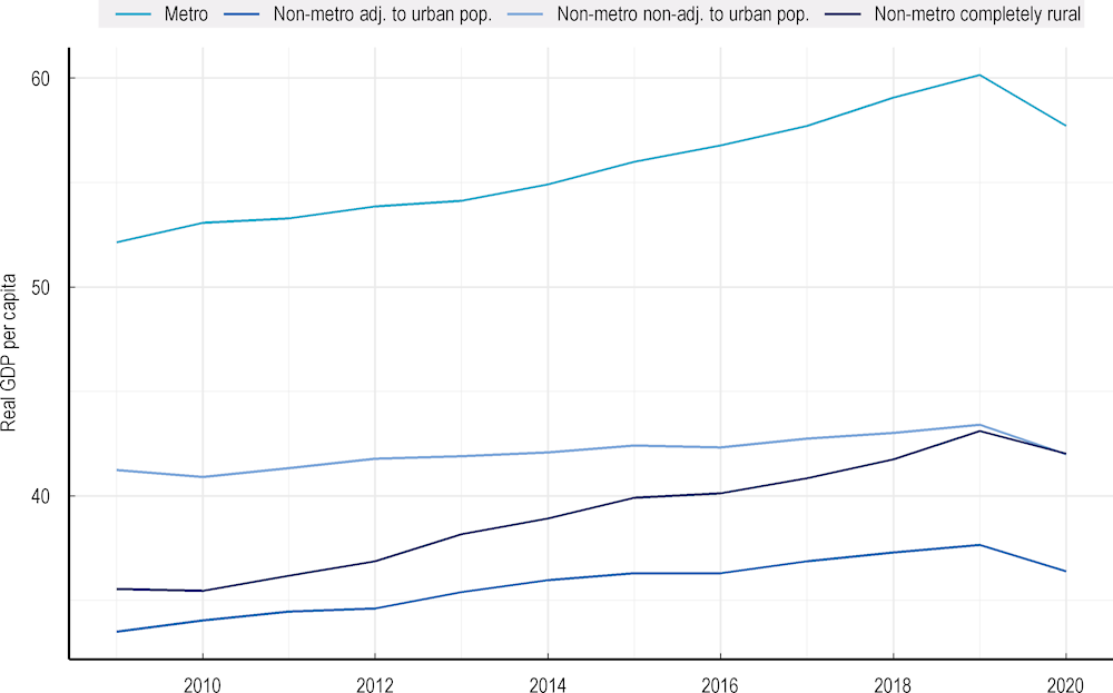
In the decade from 2010 to 2020, rural counties began to catch up to metropolitan areas in terms of per capita GDP. Since 2019, per capita GDP in rural counties has been nearly on par with non-metro NAU counties, although still significantly below that of metro counties. In general, all regions saw a rise in absolute levels of real GDP. Between 2010 and 2020, the increase in real GDP was strongest in metro counties where it grew by 18%. GDP grew in rural counties by 16%; in non-metro AU counties by 7%; and just 3% in non-metro NAU counties (Figure 2.3). Including counties with a high share of jobs in oil and gas extraction inflates GDP per capita, in terms of level and growth, in all Non-metro and Rural areas, but does not alter the converging dynamic between rural counties and non-metro NAU counties. Lastly, COVID-19 halted the upward trend for all types of counties, with metro counties decreasing the most on a per capita basis in 2020.
Figure 2.3. Real GDP per capita, 2010 to 2020
Note: Extraction-dependent counties are excluded from analysis. The four categories refer to metropolitan areas; non-metropolitan areas adjacent to urban populations; non-metropolitan areas non-adjacent to urban populations; non-metropolitan areas that are completely rural. They are further elaborated in Table 2.1.
Source: BEA (2022[8]), Regional Economic Accounts, https://www.bea.gov/data/economic-accounts/regional; U.S. Census Bureau (2022[7]), American Community Survey Data, https://www.census.gov/programs-surveys/acs/data.html.
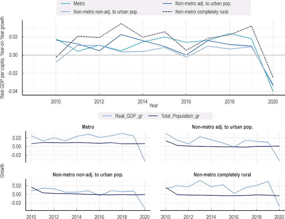
Rural counties possessed the strongest GDP growth across the decade, taking into consideration changes in population. Between 2010 and 2020, per capita GDP growth averaged 1.5 % per year in rural counties, demonstrating a resilient recovery after the financial crisis. This was followed by metro counties (0.9%), non-metro AU counties (0.8%), and non-metro NAU counties (0.2%) (Figure 2.4, top). Considering the total economy, a mini-recession was observed in 2016 owing to conditions described above, and specifically to decreased private inventory investment and in non-residential fixed investment and slowdowns in personal consumption expenditure, in residential fixed investment, and in state and local government spending (BEA, 2017[12]). All regions were affected across the United States, with non-metro NAU even experiencing a temporary, but mild, contraction.
Figure 2.4. Real GDP per capita growth (top) and its components (bottom), 2010 to 2020
Note: Extraction-dependent counties are excluded from analysis. The four categories refer to metropolitan areas; non-metropolitan areas adjacent to urban populations; non-metropolitan areas non-adjacent to urban populations; non-metropolitan areas that are completely rural. They are further elaborated in Table 2.1. Bottom figures refer to “real GDP growth” and “total population growth”.
Source: BEA (2022[8]), Regional Economic Accounts, https://www.bea.gov/data/economic-accounts/regional; U.S. Census Bureau (2022[7]), American Community Survey Data, https://www.census.gov/programs-surveys/acs/data.html.
Analysis of the components of per capita GDP reveals that its dynamics are largely driven by changes in output, against a less marked change in population (Figure 2.4, bottom). At the same time, metro counties’ rise in GDP level is accompanied by a concurrent rise in their population, resulting in a nearly perfect correlation (0.98). For rural counties, GDP increased against a declining population, resulting in a clear negative correlation (-0.72). This result gives rise to the interpretation that GDP and population are linked in metro counties, while decoupled for rural counties. The latter might be explained by the fact that isolated rural communities are more self-reliant in terms of sourcing inputs and hiring workers, and have thereby developed economies that are less labour-intensive, stable to population changes, or have invested in sufficient capital stock to be relatively independent. For the remaining non-metro counties, the relationship between GDP and population is positive (0.5 for non-metro AU counties and 0.7 for non-metro NAU counties).
Rural counties witnessed consistent depopulation between 2010 and 2020, averaging a yearly decline of 0.06%. Other regions saw population growth: highest in metro (0.78%), followed by non-metro NAU counties (0.19%), and non-metro AU counties (0.14%).9 The loss of population mechanically contributes to gains in per capita GDP in rural counties. However, as will be discussed later, there is evidence to suggest that rural counties are compensating for the lack of workers and a shrinking work force by devising innovative solutions such as upgrading and adopting new technologies, resulting in gains in productivity and ultimately output.
An international comparison reveals that the regional GDP gap in the US is higher than the average, which includes 25 other OECD countries. The GDP gap, as measured by the difference in real GDP per capita between the top 20% and bottom 20% of regions, averaged USD 30 890 across the 26 countries where regional data is available between 2008 and 2020 (Figure 2.5). The US gap stood at USD 34 551, or 12% above the average, larger than 18 countries and smaller than 7 others. Taking the size of GDP into account, the US gap is 62% of its GDP per capita, against an international average of 85%. Of the regions reported to be in the top 20% of GDP, 70% are in metropolitan regions (MR-L and MR-M) and 26% are in rural regions (NMR-R), against 26% and 61% for the bottom 20%. In top-performing rural counties, most are characterised by a strong mining, quarrying, oil and gas extraction sector, as well as retail trade. Caution should be taken in making comparisons of these figures with the rest of the report: the OECD typology focuses on defining administrative regions by their access to cities (Annex Box 2.A.1) and is used here as an exception to facilitate international comparison.
Figure 2.5. International comparison of geographical gap of GDP per capita, average of 2008‑20
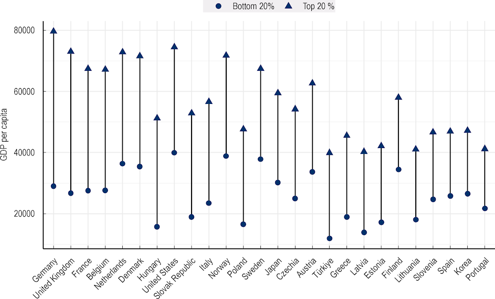
Note: For international comparison, the classification of all regions used in this analysis is the OECD Typology for Access to Cities, departing from the rest of the report which uses a simplified USDA rural-urban classification. The graph shows the gap between the mean GDP per capita of the top and bottom 20% of the countries’ regions as measured by their respective GDP per capita. Top (bottom) refers to top (bottom) 20% regions with the highest (lowest) GDP per capita levels with populations adding up to at least 20% of the national population. The x-axis is ordered by the size of the income gap, a measure of regional disparity. Extraction-dependent regions are included for all countries.
Source: OECD (2023[13]), Regional Indicators, https://stats.oecd.org/ (accessed on 15 June 2023).
In terms of labour productivity, metro counties were the most productive between 2010 and 2020, with rural counties quickly converging (Figure 2.6, top). A common explanation for the productivity gap is that metro counties, naturally benefitting from a larger pool of workers and agglomeration (Angel and Blei, 2016[14]), have the right preconditions for high productivity. In addition, the composition of sectors is such that many patent-producing firms are located in metro counties. Despite not having these advantages, rural counties nonetheless forged a path of convergence in productivity level similar to that of metro counties. Similarly, Non-metro AU and Non-metro NAU observed a trend of convergence in the decade, with the former catching up, although it remains the least productive type of area. As an aside, we note with interest that had extraction-dependent counties been included, rural areas would have surpassed metro in productivity level in 2018, and would have continued to rise.
The phenomenon of catching up for rural counties is due to its persistently strong growth in the entire period from 2010 to 2020. This group, in the years following the 2008 financial crisis, observed the highest growth among all territories between 2009 and 2014, averaging an annualised rate of 1.5% (Figure 2.6, bottom). This momentum only continued in the second half of the decade, strengthening to 1.7%. On the other hand, metro’s relatively tepid productivity growth is characteristic of the general productivity slowdown seen in OECD economies (Andrews, Criscuolo and Gal, 2016[15]) and also in the United States (BLS, 2021[16]). Metro counties’ performance eventually gathered pace in the 2015-20 period, increasing its annualised productivity growth from 0.4% to 1.2%.
Non-metro AU’s productivity also caught up to non-metro NAU, although at a slower rate. Non-metro AU productivity had relatively stable growth at 1.3% (annualised) during the 5-year period after the financial crisis, before dulling to 0.7% during 2015-20. Meanwhile, Non-metro NAU performance remained tepid throughout the decade.
Figure 2.6. Labour productivity (top) and annualised growth (bottom), 2009 to 2020
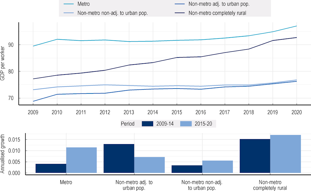
Note: Extraction-dependent counties are excluded from analysis.
Source: BEA (2022[8]), Regional Economic Accounts, https://www.bea.gov/data/economic-accounts/regional.
Rural counties are not homogenous. They tend to either be particularly productive, or particularly unproductive. Rural areas have the largest share of labour-productive (counties in the top quintile, and therefore ranked in the top 20 percent of all counties based on productivity) counties and simultaneously the largest share of labour-unproductive (least productive quintile) counties among all of the different classifications of counties (Figure 2.7, right). Defined as those in the top and bottom quintile of labour productivity across the US, more than a quarter of the highest-performing, and more than a quarter of the lowest-performing, counties were rural in 2020. This dynamic was also observed in 2010, although it is clear that rural counties have progressed in terms of their share of top-productive firms and decreased their share of bottom-productive firms. This result has been adjusted for extractive industries, which are most common in rural regions.
The spatial distribution of labour-productive firms generally remained stable between 2010 and 2020. The share of the most productive counties (quintile 5) increased in rural and non-metro AU counties and decreased elsewhere. That top-productive counties are more often rural than metro could explain the rise in labour-productivity in Figure 2.6, and the increasing share of top-productive firms of non-metro AU counties could explain the catch-up to non-metro NAU counties. We also note that the least productive counties (quintiles 1 and 2) saw a slight increase in metro area between 2010 and 2020.
Figure 2.7. Distribution of labour-productive counties, 2010 (left) and 2020 (right)
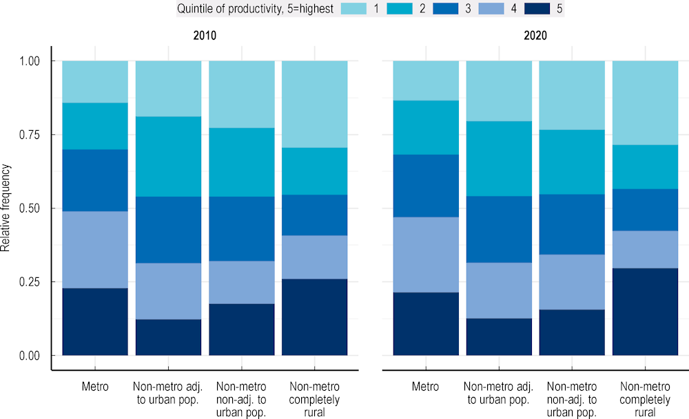
Note: Extraction-dependent counties are excluded from analysis. This figure first categorises all counties into 5 quintiles of productivity, where the 5th quintile reflects the highest level of productivity, and the 1st reflects the lowest levels of productivity. It then provides the frequency at which counties are placed into different territorial (geographical) classifications.
Source: BEA (2022[8]), Regional Economic Accounts, https://www.bea.gov/data/economic-accounts/regional.
Sector dynamics across US territories
In 2020, the top three industries contributing to rural counties’ private GDP were finance, insurance, and real estate (24%), agriculture (23%), and manufacturing (13%). Agriculture, in particular, saw the highest increase in the economic share between 2010 and 2020, while manufacturing shrunk, in line with the well‑documented decline in rural manufacturing (Charles, Hurst and Schwartz, 2019[17]). Part of this decline is the relocation of the sector to non-metro AU, which saw an increase between 2010 and 2020 (Figure 2.8).
In metro counties, the top contributing sectors are finance, insurance, real estate (23%), professional services (16%), and manufacturing (13%). These rankings remain unchanged from 2010. In particular, rural counties observe 8 industries which have shrunk since 2010, being offset by a strong 4.8 percentage point increase in agriculture. This analysis excludes government and mining, the latter of which would otherwise occupy 15% of the rural economy in 2010, nearly doubling to 27% in 2020, skewing the result for other sectors.
In metro counties, while remaining a top-contributing industry, finance, insurance and real estate has shrunk by 0.9 percentage point, and manufacturing by 1.1 percentage point in the decade. This was offset by a 2.0 percentage point gain in professional services, and notably information (2.7 percentage point). Non-metro NAU counties and non-metro AU counties observed manufacturing as the predominant industry in 2020, even registering an increase of 2.4 percentage points and 0.4 percentage points, respectively, from 2010. The structure of the economy in all regions appeared stable in the decade from 2010 to 2020, excluding mining.
Figure 2.8. Share of GDP by industry in 2010 and 2020
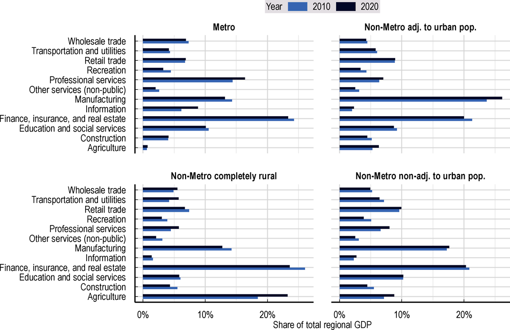
Note: Units are at constant 2012 USD. Only private sector firms are considered. Mining and quarrying are excluded from this analysis. Indeed, calculating total regional GDP would have a distortion effect on other sectors. Industries included farm employment and private non-farm employment, as defined by the Bureau of Economic Analysis. Sectors are abbreviated for brevity; see Annex Box 2.A.1 for details. Counties with no Real GDP data due to confidentiality or lack of availability have been excluded from analysis; as such, underestimation is expected.
Source: BEA (2022[8]), Regional Economic Accounts, https://www.bea.gov/data/economic-accounts/regional.
In rural counties, the top employers are in education and social services, manufacturing, and retail trade. Thus, the notion that rural areas are necessarily agrarian does not hold as non-agriculture sectors employ more workers in rural areas. It has to be noted however that agriculture still employs a higher share of rural resident workers than any other region (Figure 2.9). In addition, employment from mining, oil and gas only comprised a small share (less than 5%) in all groupings. In metro counties, the top employer is by far the education and social services sector, followed by professional services (including scientific, management, administrative and waste management), and retail trade.
The ranking of these top sectors has generally been stable when compared to 2010. However, all county groupings increased their employment share in the broad tertiary (service) sector, while moving away from primary and secondary sectors (agriculture, construction, and manufacturing). Across the board, this is most notable in the increase of employment share in education and social services (including health services), professional services, and recreation. Nonetheless, the trend toward services does not account for the fact that manufacturing helps create employment in other non-tradeable sectors (Moretti, 2010[18]). In addition, high- and medium-tech manufacturing account for the lion’s share of all patents granted in the US (National Science Foundation, 2018[19]), indicating the potential that this sector brings to innovation in non-metropolitan and rural areas.
Figure 2.9. Sources of employment by sector in the United States, 2020 and 2010
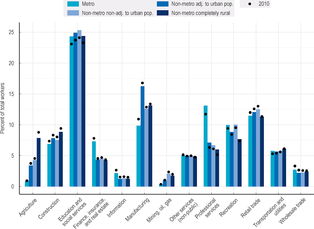
Note: Bars denote 2020 values while black dots denote 2010 values. Extraction-dependent counties are included. Sectors are abbreviated for brevity; see Annex Box 2.A.1 for details. Departing from previous analysis, this analysis is resident-based, rather than employee-based. That is, for a given county, this counts the number of people who work in a specific sector, regardless of the location of employment.
Source: U.S. Census Bureau (2022[7]), American Community Survey Data, https://www.census.gov/programs-surveys/acs/data.html.
Non-metro economies, driven by changes in rural counties, lost 0.2% of its workers between 2010 and 2020 (in absolute terms), averaging a 0.02% decline per year during the decade. This stands in contrast to metro economies which have seen increased workers between 2010 and 2020, growing on average by 1.1% each year. Breaking down the group, rural counties saw declines of 0.4% annually between 2010 and 2020, while non-metro NAU counties averaged losses of 0.04%; non-metro AU counties grew.
By sector, and adjusted for population movement, rural counties lost workers in 9 of the 12 sectors considered in the analysis between 2010 and 2020. Figure 2.10 illustrates employment changes in major sectors between 2010 and 2020. Notably, despite being a top contributor to rural GDP, which increased during the decade, the agricultural workforce declined by 1.5%. This might be due to mechanisation of the sector resulting in less labour-intensive processes, combined with general shortages of farm workers (Wang et al., 2022[20]; Hamilton et al., 2022[21]). The decrease of workers in the information sector was the most salient in rural counties, but occurred across all territories. Such decline was driven by the telecommunications sub-sector, where larger firms contracted out work to smaller firms, which depressed wages and benefits (known as “fissuring”), and long-term decline in unionisation (Schmitt and Kandra, 2020[22]; Weil, 2017[23]). Of the three sectors in rural counties which did not decline, only professional services saw substantial growth, at 12.8%, while recreation and education and social services saw negligible change.
Figure 2.10. Change in number of workers by industry, 2010-20
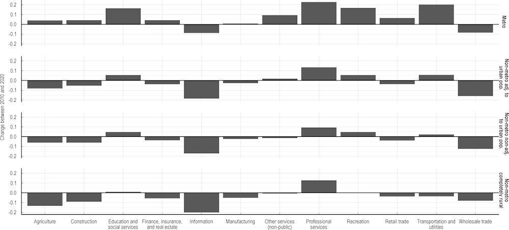
Note: Extraction-dependent counties are excluded. The changes have been adjusted for movement in the respective grouping’s population between 2010 and 2020. Sectors are abbreviated for brevity; see Annex Box 2.A.1 for details.
Source: U.S. Census Bureau (2022[7]), American Community Survey Data, https://www.census.gov/programs-surveys/acs/data.html.
Metro counties added workers in nearly all industries, which provides supporting evidence of the agglomeration of workers in metro counties. Two exceptions were found in information and wholesale trade, which saw job losses. Professional services recorded the highest growth in the decade from 2010 to 2020, at 23%, followed by transportation and utilities (20%), and recreation (17%). Agriculture observed an increase of 4% in metro counties, potentially related to the rise of urban farming or centralisation of farm business activities in urban headquarters.
The employment growth dynamics in all non-metro counties is broadly similar in the shift from primary and secondary sectors to services, although only select service sectors increased. Professional services saw the highest growth across all non-metro counties, as observed also in metro counties. Employment growth also came from recreation, education and social services, and other services (non-public). Increases in workers in these sectors were offset by drops in the remaining sectors, most markedly in information and wholesale trade.
Lastly, this analysis demonstrates that the most substantial driver of productivity change has been the improved use of resources within territories. Notably, approximately 38% of all productivity growth in the United States was due to more efficient use of resources in rural counties over the past 10 years (Figure 2.11, top). Considering all non-metropolitan regions, this was even greater at nearly two-thirds (61%).10 These types of gains are attributed in part to the capacity of rural regions to absorb innovation and upgrade resources. Investing in the upskilling of workers and firms in non-metropolitan regions will likely continue to contribute positively to aggregate productivity.
Figure 2.11. Decomposing changes in productivity
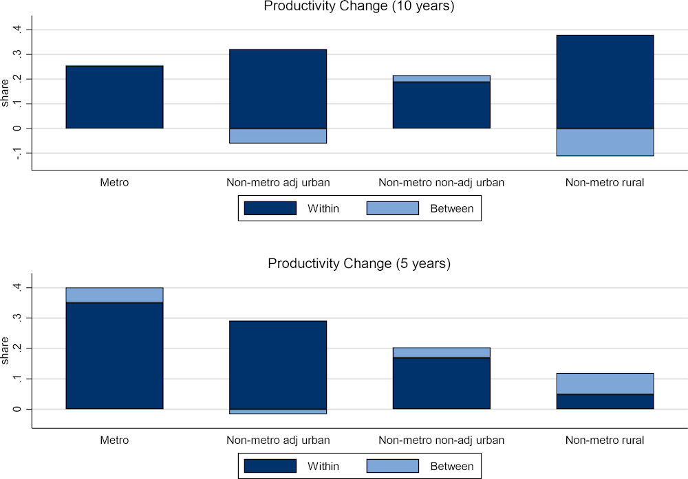
Note: There is no entry and exit of firms, as analysis is done based on county level estimates. Oil counties have been excluded. The equation decomposes (breaks) productivity down into “within” components and “between” components. The decomposition takes the following form:
.
Where and refer to economy-wide productivity and the productivity for each type of county, and is the share of employment in the type of county, i. The first term refers to the changes in the contribution of the share of employment within in each type of county to productivity, while the second component , refers to the change in overall productivity due to the reallocation of resources between each type of county. Data used is pooled and averaged by 5-year intervals. The proxies used refer to 2006-10 for 2010 estimates; 2011-15 for 2015 estimates; and 2016-20 for 2020 estimates.
Source: OECD analysis based on BEA (2022[8]), Regional Economic Accounts, https://www.bea.gov/data/economic-accounts/regional; Aggregate Labour Productivity Decomposition following McMillan, M., D. Rodrik and Í. Verduzco-Gallo (2014[24]), “ Globalization, structural change, and productivity growth, with an update on Africa”, https://doi.org/10.1016/j.worlddev.2013.10.012.
However, rural regions also experienced some offsets to these productivity gains due to reallocation of resources between territories. In the context of analysis in this section, offsets were likely, in part, due to workers leaving the territories. Non-metro AU saw a similar, but smaller, dynamic. Rural counties observed a 11% loss of productivity due to resource reallocation, while non-metropolitan AU observed a 6% loss. Surprisingly, non-metropolitan NAU counties made slight gains in productivity at 3% due to reallocation. This last gain was consistent in both 10- and 5-year growth models.
Unfortunately, in the last five years, non-metropolitan counties’ contribution to overall growth has been cut by half. Productivity growth has slowed for rural counties and picked up for metropolitan counties totalling 28% on the whole for all non-metropolitan counties (Figure 2.11, bottom).11 With more gains from reallocation than losses but much lower gains in efficiency, the last five years have been a both positive and negative for non-metropolitan regions.
Innovation in the United States
The US is a leader of innovations in firm products and processes. It often is measured at the top of rankings in standard innovation statistics such as private R&D expenditures, patent applicants and high firm-growth. In 2020, the United States logged 646 244 patent applications, of which 60%, or 388 900, were granted12 (USPTO, 2022[25]).
However, not much is known about the geography of innovation in rural areas, except for strong performance on overall patent statistics in California and New York, which are states with large populations and a high share of occupations whose innovative outcome may result in patent-filing, or strong R&D investment. As argued previously, when possible, the report adjusts measures of innovation to reflect individual characteristics of people living in different areas. As such, the rest of this section adjusts patents by the occupational structure of geographies as described in Annex 2.B and Dotzel and Wojan (2022[26]).13
Despite this more nuanced approach, the analysis is still cautious in its interpretation because it overlooks innovation in non-patented products and processes. The occupations considered inventive include jobs in the professional scientific, and management, and administrative services sectors; manufacturing sectors; and arts, entertainment, and recreation sectors; and accommodation and food services sectors. These were identified as occupations of inventors most likely to file a patent (Dotzel and Wojan, 2022[26]). For example, there are vast differences when looking at the best performing counties in terms of patents and patents per innovative occupations. While the county with the highest number of patents is Santa Clara County (CA), a metro county, the highest intensity, patents per inventive occupation (or occupation that is more likely to patent), is actually found in a rural county, in Barbour County (AL).
The analysis in this section uses data on county level from the American Community Survey 5-year estimates (ACS) (2022[7]), the Bureau of Economic Analysis’ (BEA) Regional Economic Accounts (2022[8]), firm counts from County Business Patterns (CBP); information on patents from the United States Patent and Trademark Office (USPTO); and innovative occupations from Dotzel and Wojan (2022[26]). Because the latter is only available for 2015, we display mostly cross-sectional evidence. For ease of interpretation, territorial (geographical) classifications are more frequently grouped into metropolitan and non‑metropolitan counties.
Box 2.1. The relationship between patents, innovation and economic growth
The relationship between patents and economic growth has not been conclusive. Early Schumpeterian models suggest that growth is mainly driven by innovation, which replaces and improves upon previous capital used in production, thereby making companies more productive. Innovation is therefore located at the heart of economic development and facilitates aggregate economic growth (Nelson and Winter, 1982[27]). In models of endogenous growth, productivity improvement is traditionally due to spending on research and development, which enhances output (Romer, 1990[28]; Romer, 1994[29]). The key insight is that knowledge spillovers, because of the long-run non-excludability and non-rivalry of ideas (i.e. patents expire), is one of the primary drivers of growth. Nonetheless, firms are incentivised to generate new ideas since in the short run patent protection endows them the exclusive right to profit from innovation.
Nevertheless, empirically this result has been contested. A strand of the literature using country level data on patents shows a significant impact of patents on growth (Akçomak and ter Weel, 2009[30]; Hasan and Tucci, 2010[31]). This literature highlights the importance of knowledge creation and corroborates the theory of endogenous growth. However, it has been argued and shown empirically that patents can also have no strong effect on growth (Sweet and Eterovic, 2019[32]; Blind, Ramel and Rochell, 2022[33]). This argument highlights several weaknesses of patents as a measure of innovation.
First, each sector and even each firm has their specific patenting rules and quality controls. Research shows that patent growth is also associated with subsequent growth of R&D in the medical and optical equipment industry as well as in the electrics and electronics industry. Neither of these effects can be found for both the chemicals and the transport equipment industries (Buerger, Broekel and Coad, 2012[34]). Second, not all inventions are innovative. A patent becomes an innovation if it is first “available to potential users” and second “brought into use” (OECD/Eurostat, 2018[35]). For instance, about one-third of patents are not utilised and patenting in specific sectors may be viewed as a strategic measure to block competitors (Giuri et al., 2007[36]). Therefore, it might be knowledge diffusion rather than knowledge creation which drives productivity growth.
Source: Nelson, R. and S. Winter (1982[27]), An Evolutionary Theory of Economic Change, Harvard University Press, Cambridge, Mass; Romer, P. (1994[29]), “The origins of endogenous growth”, Journal of Economic Perspectives, Vol. 8/1, pp. 3-22, https://doi.org/10.1257/jep.8.1.3; Romer, P. (1990[28]), “Endogenous technological change”, Journal of Political Economy, Vol. 98/5, pp. 71‑102; Hasan, I. and C. Tucci (2010[31]), “The innovation-economic growth nexus: Global evidence”, https://doi.org/10.1016/j.respol.2010.07.005; Akçomak, İ. and B. ter Weel (2009[30]), “Social capital, innovation and growth: Evidence from Europe”, https://doi.org/10.1016/j.euroecorev.2008.10.001; Sweet, C. and D. Eterovic (2019[32]), “Do patent rights matter? 40 years of innovation, complexity and productivity”, https://doi.org/10.1016/j.worlddev.2018.10.009; Blind, K., F. Ramel and C. Rochell (2022[33]), “The influence of standards and patents on long-term economic growth”, https://doi.org/10.1007/s10961-021-09864-3; Buerger, M., T. Broekel and A. Coad (2012[34]), “Regional dynamics of innovation: Investigating the co-evolution of patents, research and development (R&D), and employment”, https://doi.org/10.1080/00343404.2010.520693; OECD/Eurostat (2018[35]), Oslo Manual 2018: Guidelines for Collecting, Reporting and Using Data on Innovation, 4th Edition, https://doi.org/10.1787/9789264304604-en; Giuri, P. et al. (2007[36]), “Inventors and invention processes in Europe: Results from the PatVal-EU survey”, https://doi.org/10.1016/j.respol.2007.07.008.
Individuals as drivers of innovation
Metropolitan counties on average had the highest patent intensity in 2015 (Figure 2.12).14 There are on average 13.2 patents per 1 000 innovative occupations in metropolitan counties, while this ratio is 5.6 on average in rural counties. This pattern is similar for the share of innovative occupations of the total workforce within counties. Within metro counties’ innovative workforce, over 5% are patent-producing, compared to 3.5% in non-metropolitan AU counties, 2.8% in non-metropolitan NAU counties, and 2.6% in rural counties.15 By construction, the number of innovative occupations as a share of the total workforce is strongly correlated with patent output (Figure 2.12, Panel B).
Figure 2.12. Innovation rates across counties, 2015
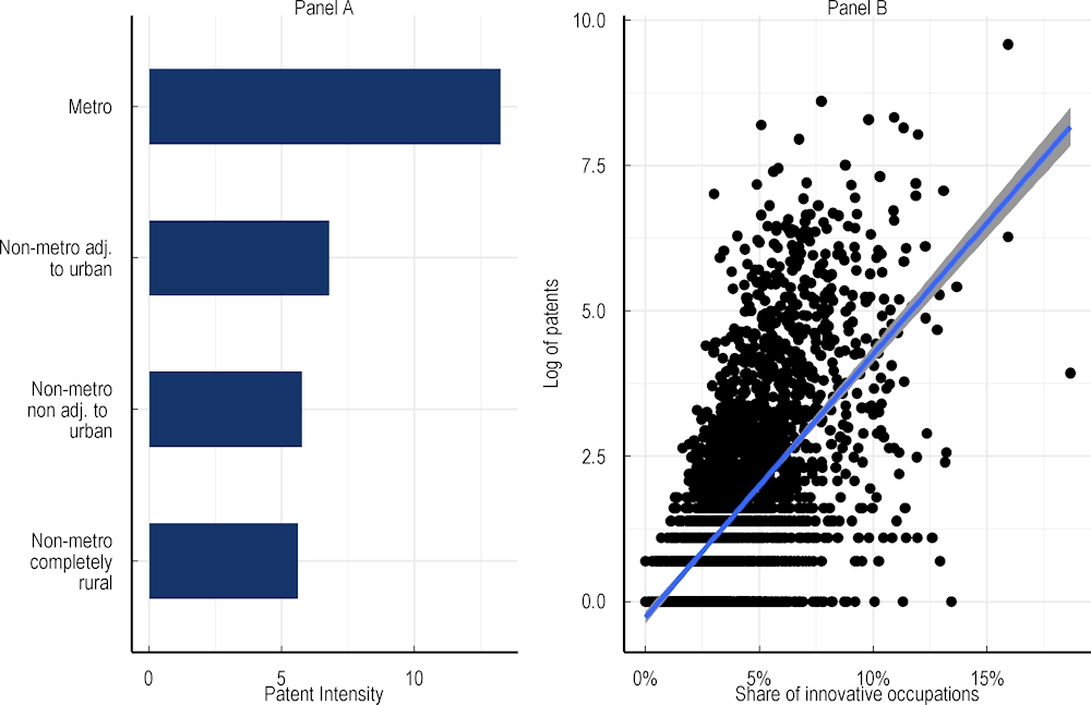
Note: Panel A displays the average patent intensity by county classification (Table 2.1). The patent intensity is computed by dividing the number of patents by the number of innovative occupations in a given county. Panel B shows the correlation between the numbers.
Source: Dotzel, K. and T. Wojan (2022[26]), “An occupational approach to analyzing regional invention”, https://ncses.nsf.gov/pubs/ncses22202; United States Patent and Trademark Office.
Counties with larger shares of inventive workers tend to have high levels of employment, but they do not necessarily have higher productivity (Figure 2.13, Panel A and B).16 Within metropolitan counties, the highest quintile of counties with high shares of innovative occupations accounts for nearly 75% of all employment (Figure 2.13, Panel A). In contrast, in non-metropolitan AU counties, non-metropolitan NAU counties and rural counties less than 50% of workers are employed in counties with high shares of innovative occupations. In other words, metropolitan counties with more innovative occupations tend to also have the largest share of workers. However, in non-metropolitan counties, innovative occupations are not densely clustered into counties that have a larger labour pool.
The existence of individuals with the proclivity to participate in high-tech (and patentable) innovation does not necessarily align with the productivity outcomes. Output per worker (productivity) is roughly equally distributed among all county classifications, except for completely rural counties where the middle rank of counties based on patent intensity carries a larger share of output per worker. This suggests that innovative occupations are not strongly associated with labour productivity and that some rural counties are managing their resources more effectively, for instance by employing labour in a more productive way.17
Figure 2.13. Employment and productivity across the innovation distribution
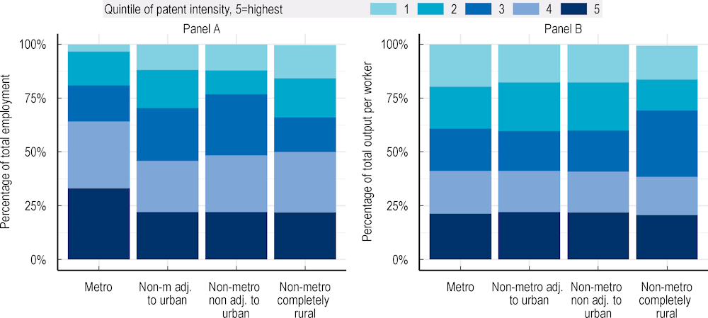
Note: Quintiles are based on the distribution of innovative occupations within county classification. The colours refer to the quintile whereas the size of the bar indicates the share of the respective quintile of total employment and output per worker for each county class. Patent statistics are available for 2015, and ACS data are based on 2000-15 data.
Source: U.S. Census Bureau (2022[7]), American Community Survey Data, https://www.census.gov/programs-surveys/acs/data.html; BEA (2022[8]), Regional Economic Accounts, https://www.bea.gov/data/economic-accounts/regional; Dotzel, K. and T. Wojan (2022[26]), “An occupational approach to analyzing regional invention”, https://ncses.nsf.gov/pubs/ncses22202.
Education is often considered an important determinant of high-tech innovation, but the relationship between higher education and innovation is not exactly the same in metropolitan and non-metropolitan areas. Panel A of Figure 2.14 demonstrates the point. First, the share of those in tertiary education is lower in non-metropolitan areas than in urban areas. Nevertheless, increasing the share of workers with tertiary education leads to an increase in the ratio of the number of patents to innovative occupation for both metro and non‑metro counties respectively.18 Overall, a 1% percentage point increase in the share of the workforce with tertiary education is associated with a 2.1 (2.1 patents per 1 000 relevant occupations) increase in patent intensity in metro and a lower, 1.1 increase in patent intensity in non-metro counties. After the threshold of around 20 percent of the workforce with tertiary education, the total benefit of increasing the share of tertiary education labour force becomes less clear (i.e. estimates become noisy with larger standard errors) and is a lower magnitude for non-metropolitan areas. This finding suggests that increasing the stock of highly educated workers alone in non-metropolitan areas does not have the same impact (despite both being still positive), in non-metropolitan areas, as compared to those in metropolitan areas. The level of education of the labour market is particularly relevant for innovation in non-metropolitan areas that benefit from a higher educated workforce, but it may miss a local focus on the supply of education courses to best fit local markets (see Chapter 4).
Despite mixed findings on innovation, investing in the workforce is still clearly positive for non-metropolitan and metropolitan counties alike. For both metropolitan and non-metropolitan counties, there is a positive relationship between government spending in education per capita and productivity. However, the effects of government spending are marginally more positive in non-metropolitan areas. Increasing governmental spending on education by 1% in non-metropolitan areas is associated with an increase productivity by 0.5%, as compared to a 0.3% increase in metro counties.
Figure 2.14. Education and innovation
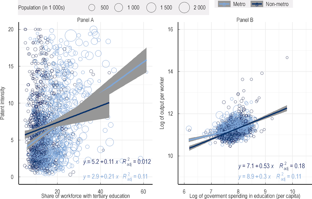
Note: Patent intensity is computed by dividing the number of patents by the number of innovative occupations in a given county. The workforce with tertiary education has been denominated by total workforce. Government spending on education has been denominated by total population. Outliers in patent intensity have been excluded in all graphs. Observations are from 2015.
Source: U.S. Census Bureau (2022[7]). American Community Survey Data. https://www.census.gov/programs-surveys/acs/data.html; BEA (2022[8]), Regional Economic Accounts, https://www.bea.gov/data/economic-accounts/regional; Dotzel, K. and T. Wojan (2022[26]), “An occupational approach to analyzing regional invention”, https://ncses.nsf.gov/pubs/ncses22202.
Firm-based innovation: Competition, higher education and research institutions
If individuals are drivers of innovation, firms are the mechanisms through which they instrumentalise their ideas. Framework policies regulating firm activities related to competition, finance and human capital are important factors for encouraging innovation (Aghion et al., 2001[37]; Andersson et al., 2009[38]; Grossman and Helpman, 1990[39]). In many cases, the establishment of a new firm implies finding a new product or process that can bring new opportunities to the firm itself or the market it serves. Therefore, more firm activity may both be driving innovation directly, and indirectly through competition, spillovers or simply more specialised services.
There is a strong potential for innovation through encouraging new entrepreneurship. In OECD countries, there is ample evidence suggesting that start-up entrepreneurs tend to be innovative. A portion of start‑ups are also highly productive (Freshwater et al., 2019[40]; Hall, 2011[41]; OECD, 2013[42]; 2019[43]). Higher start‑up rates and creative destruction (firm churning, or firm birth and death rates) are often an indicator of healthy, evolving and innovative economies (2017[44]). Moreover, young firms such as start‑ups undertake riskier innovation activities that may yield greater performance benefits or greater losses (Coad, Segarra and Teruel, 2016[45]; Breschi, Lassébie and Menon, 2018[46]).
At the aggregate level, the growth in number of firms in non-metro counties is low, while there is a strongly positive growth for metropolitan firms after 2014 (Figure 2.15, top). At the same time, patent growth follows a decreasing trend in non-metropolitan counties and has been stagnating in metropolitan counties since 2010 (Figure 2.15, bottom). This suggests that the relationship between new firm growth and patents is not monotonous (constant), especially across county classifications.
Figure 2.15. Growth rate of firms and patent intensity
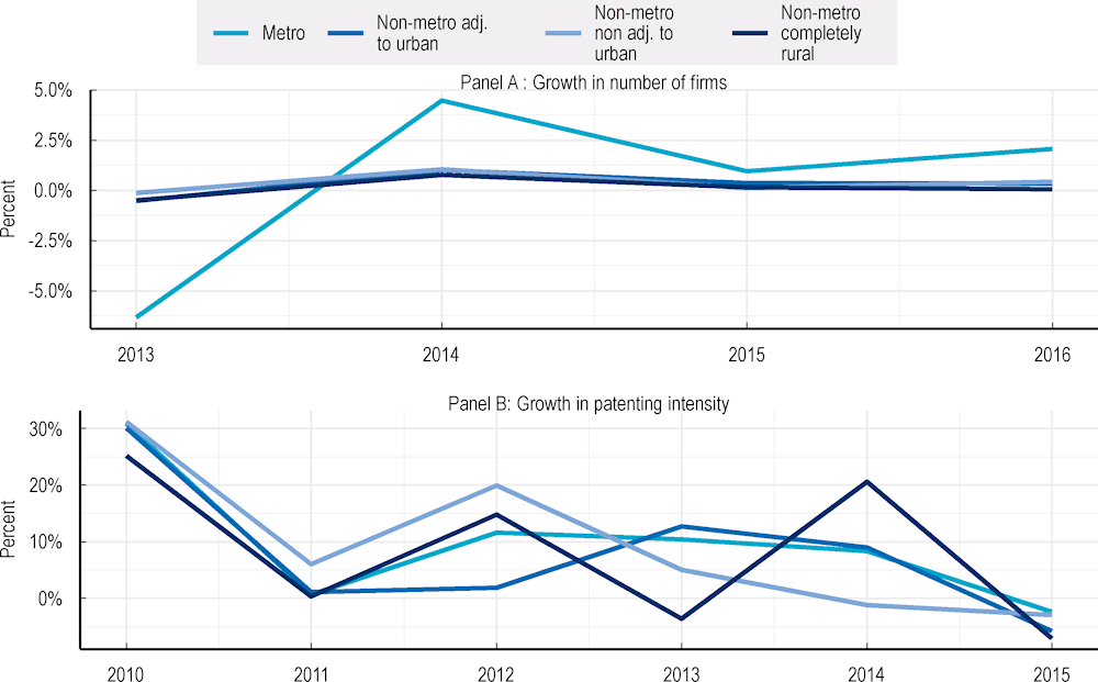
Note: Growth rate of aggregate firms and patents by county classification. Panel A shows the growth rate of the number of firms by county class. Panel B shows the growth rate of patents by county class.
Source: County Business Patterns Data, https://www.census.gov/programs-surveys/cbp/data.html ; United States Patent and Trademark Office; Dotzel, K. and T. Wojan (2022[26]), “An occupational approach to analyzing regional invention”, https://ncses.nsf.gov/pubs/ncses22202.
Competition is often considered good for innovation and growth, yet imperfect competition can create unfair advantages. In rural counties, more firm activities are associated with higher patent intensity. The more firms there are per thousand workers, the higher the patent intensity. In other words, an increase in firm density is positively correlated with patent intensity (Figure 2.16, Panel A).19 The top 25 percentile of rural counties with the highest clustering of firms average 2.6 patents per thousand inventive workers. This number drops by half in the counties with the least firms per thousand workers in rural counties. For metro counties this relationship is the opposite. There are approximately 1.5 fewer patents per inventive worker in the counties with the highest firm intensity as compared to counties with the lowest levels of firm intensity. While those metro counties in the first, second and third quartile of the firm distribution have rather similar patent intensities, those with the highest number of firms per 1 000 workers have a lower patent intensity. Assuming that industrial composition of firms remains constant across regions, this might indicate that there is a level of saturation of firm intensity associated with patent intensity in metro counties, but not in rural counties.
Figure 2.16. Firms, business associations and patent intensity
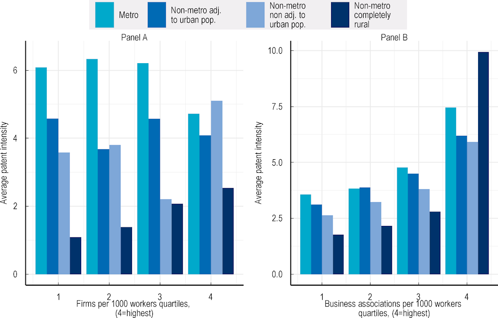
Note: Counties have been ranked by their position and the distribution of firms per 1 000 workers across the US. The bars indicate the average patent intensity by county class within their respective quartile. The analysis is based on data on number of business associations and patents in 2015.
Source: U.S. Census Bureau (2022[7]), American Community Survey Data, https://www.census.gov/programs-surveys/acs/data.html; U.S. Census Bureau (2021[47]) County Business Patterns Data, https://www.census.gov/programs-surveys/cbp/data.html ; United States Patent and Trademark Office; Dotzel, K. and T. Wojan (2022[26]), “An occupational approach to analyzing regional invention”, https://ncses.nsf.gov/pubs/ncses22202.
Higher firm intensity might be accompanied by higher spill-over effects, especially in rural counties. Either more firms attract more productive and educated workers or there are general knowledge spill-overs reducing the costs to innovate. In high tech sectors clustered in metro counties a high level of existing firms and patent thickets might hamper more innovation (Hall, von Graevenitz and Helmers, 2020[48]; Delgado, Porter and Stern, 2014[2]). If competition is high and markets are rather saturated, the willingness to innovate might be reduced since after a certain level, competition decreases potential profits. Moreover, the adverse relationship between firm intensity and innovation across rural and metro counties could be due to different types and cost structures of inventions. Differing characteristics of firms and industries across county classes (see Figure 2.8) and difficulties in access to legal services for filing patent procedures might explain this pattern further (Buerger, Broekel and Coad, 2012[34]).
In addition to firm competition, access to business networks such as business associations can help transfer knowledge between firms, and therefore contribute to an enabling environment for innovation. These associations tend to help navigate barriers to entering markets and support the private sector’s dialogue with government. Business associations are positively associated with innovation across all county classifications, and even more so for rural counties (Figure 2.16, Panel B).
Business associations perform a wide range of tasks (collective bargaining, self-regulation, representation, and lobbying) usually managing the relations between states and firms. Thus, they can play a crucial role in improving access to external knowledge, building mutually beneficial relationships, and commercialising the internal knowledge. They can directly support innovation in businesses in particular where policymaking impacts funding of R&D, technological development and innovation (Koschatzky et al., 2014[49]). Moreover, business associations facilitate the transmission of knowledge for its members. For example, in the automotive industry in Portugal it has been shown that business associations have played an important role in the transfer of knowledge and technology between project stakeholders (Carvalho and Moreira, 2015[50]).
Firm-based innovation is also often associated with spending on Research and Development (R&D). However, the effect of spending in research and development on patent intensity also differs between metro and non-metro counties (Figure 2.17). While the effect of R&D on patent intensity is positive in non-metro counties, there is a zero correlation in metro counties. For every 1% increase in R&D spending, the patent intensity increases by 0.7 units in non-metro counties while it is close to zero, and more spurious in metro counties.20 This might reflect the fact that R&D spending in non-metro counties faces less saturation compared to what is observed in other OECD countries (OECD, 2022[6]). Research expenditure can be more effective in places when the cost of innovating is lower, in particular when levels of R&D spending are at a lower, implying lower entry, barriers and marketing costs. However, rural counties with positive patent intensities and no R&D spending do in fact exist. This points to the fact that innovation in some rural counties may not be as connected to R&D spending as those in metropolitan counties and suggests the assertion that knowledge diffusion is a driver of innovation in non-metropolitan regions. In this case, rural innovation is simply less dependent on the direct effects of R&D.
Figure 2.17. Research and development spending and patent intensity
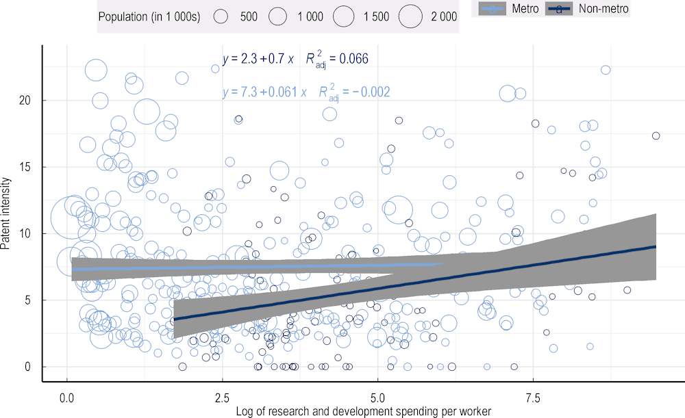
Note: The patent intensity is computed by dividing the number of patents by the number of innovative occupations in a given county. All other variables have been denominated by total employment. Counties with no patents and outliers in patent intensity have been excluded in all graphs.
Source: U.S. Census Bureau (2022[7]), American Community Survey Data, https://www.census.gov/programs-surveys/acs/data.html; BEA (2022[8]), Regional Economic Accounts, https://www.bea.gov/data/economic-accounts/regional; United States Patent and Trademark Office; Dotzel, K. and T. Wojan (2022[26]), “An occupational approach to analyzing regional invention”, https://ncses.nsf.gov/pubs/ncses22202.
Promoting equitable opportunities for innovation
Innovation is both the predecessor of growth and employment and of job loss and structural change. It happens in different ways. Innovation can create opportunities, but also exacerbate pre-existing inequalities. For example, wage inequality among top earners is associated with innovation (Aghion et al., 2018[51]). However, in the United States, growth in aggregate income by top earners is continuing to create inequalities. Among top income earners, white people have continued to increase incomes, while Black top income earners have not seen incomes progress as rapidly (Rinz and Voorheis, 2023[52]).
While some level of inequality is useful for innovation, too much inequality can hinder equitable access to opportunities and reinforce pre-existing barriers, leading to a fall in dynamism in the economy. While competitive forces may be driving top income growth through innovation, the average income earner may not experience the same benefits to innovation. Other kinds of innovation can also lead to a reduction in wage inequality over time (social mobility), in particular when it comes from new entrants (start-up entrepreneurs) to the market (Aghion et al., 2018[51]). Taking into consideration how innovation and entrepreneurship policies can promote equitable opportunities is often a target for policymakers focused on regional development or those operating in districts or states with a large constituency in rural areas, and can help address worsening geographical divides.
Diversity and interactions between individuals enable innovation (Crescenzi, Nathan and Rodríguez-Pose, 2016[1]). Social and professional networks are an important mechanism with which to diffuse knowledge. Networks with new ideas and opportunities develop as individuals from different backgrounds exchange ideas and resources. Diversity in management has been found to be an economic asset. It also generates social benefits: some studies find evidence of a “diversity bonus” for innovation in firms that had more diversity in management, providing better access to international markets, and encouraging entrepreneurship (Nathan and Lee, 2013[53]).
Diversity in all forms can foster the creation of new ideas and solutions, while reinforcing equity (Nathan and Lee, 2013[53]). However, traditional economics do not often directly take into consideration the diversity of rural challenges related to intersectionality between demographic and geographical diversity to promote inclusive opportunities (Henry-Nickie and Seo, 2022[54]). One point of strength in the United States is active measures to encourage diversity in the workforce, including in terms of minorities. For example, the EDA has investment priorities based on equity in grant-making, which includes traditionally underserved populations, including but not limited to women, Black, Latino, Indigenous and Native American persons, Asian Americans and Pacific Islanders, or critically, geographies that have a systematic lack of equitable access such as those on Tribal lands, or those that are classified as Persistent Poverty Counties (EDA, n.d.[55]).
While research is still scarce on ethnic diversity, studies on diversity in workplaces suggest more innovative group outcomes (Van der Vegt and Janssen, 2003[56]; Goodman, 2013[57]). However, US-born minorities, such as Asian, African, Hispanic and Native Americans, account for 32% of the native-born population, but just 8% of US-born innovators. African Americans comprise 13% of the native-born population, yet only 0.5% of US-born innovators according to the Information, Technology and Innovation Foundation (Nager et al., 2016[58]). For rural communities with relatively smaller populations, national minorities can become local majorities creating additional different challenges on activating diversity and accessing resources for innovation and entrepreneurship.21 In some cases, historical discrimination is some areas has persisted over time, thus stifling opportunities for growth and well-being.
Innovation, inequalities and demographic change
Innovation is driven by people and skills. Promoting access to skills and skills diversity is therefore a primary concern for many regional and rural governments looking to encourage innovation. As in other OECD countries, rural regions are faced with an aging workforce, challenges to engage with youth, and often increasing discrimination in the workforce related to gender, race and or migration status (OECD, 2019[59]). Efforts to promote equity in access to opportunities through innovation and entrepreneurship programmes should take into consideration the demographics of non-metropolitan regions in addressing these challenges. Given the importance of promoting innovation and entrepreneurship through a well‑being approach, this sub-section explores trends on inequality, demographics and population change for innovation.
Trends in inequalities
Comparing the United States to 18 OECD countries22 where disposable household income is available at the TL3 level, we find that overall inequality was higher in the US in 2019, at 0.13, compared to the OECD average of 0.11 (Figure 2.18, right). In metro and non-metro AU regions,23 we observe lower inequality in the US as compared to OECD countries. However, in non-metro NAU regions and rural regions, inequality is starkly higher in the US than in OECD countries, with non-metro NAU regions surpassing the OECD average by over 2.5 fold. However, such analysis aggregates county level variations within regions.
Based on more disaggregate data, in the United States today, the highest level of household income inequality among wage earners is found in metropolitan and completely rural counties (Figure 2.18, left). However, notably, in the last five years (2015 to 2020) inequality in rural counties has fallen, while it continued to grow in metropolitan counties. Between 2010 and 2020, the rise in income inequality as measured by the Gini coefficient24 (Figure 2.18, left) is also accompanied by the rise in real GDP per capita in most counties (Figure 2.3). In general, overall inequality (dotted red line), driven by metro counties, showed an upward trend.
Figure 2.18. Gini coefficient on county household income, 2009 to 2020 (left), and international comparison, 2019 (right)
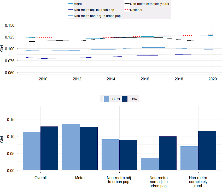
Note: Extraction-dependent counties are excluded from analysis. On the right, the OECD averages are for 2019 and include the following countries: Czechia, Germany, Denmark, Estonia, Hungary, Ireland, Israel, Iceland, Japan, Korea, Lithuania, Latvia, Norway, New Zealand, Sweden, Slovenia, Slovak Republic, the United Kingdom. Disposable household income on the US at the county level originated from the 5-Year American Community Survey while that of others, at the OECD TL3 level, originated from the OECD Regional Statistics Database. Date in both graphs is based on TL3 regions and classified into the OECD’s typology of small administrative regions (TL3) based on accessibility to metropolitan areas. The category labels are adapted from the OECD’s typology based on access to cities to similar labelling of the RUCC typologies for ease of interpretation and comparability with other figures. Non-metro adjacent to urban population category refers to the OECD’s non-metropolitan regions with access to a metropolitan areas (NMR-M) category. Non-metro non-adjacent to urban population category refers to the OECD’s non-metropolitan regions with access to a small- and medium-sized city (NMR‑S) category. Non-metropolitan completely rural category refers to the OECD’s non-metropolitan remote regions (NMR-R) category.
Source: U.S. Census Bureau (2022[7]), American Community Survey Data, https://www.census.gov/programs-surveys/acs/data.html; OECD (2022[60]), Regional Statistics, https://www.oecd.org/regional/regional-statistics/.
There have been broad improvements in reducing inequality in rural counties from 2009 to 2020. In contrast, to the trend in metro counties, rural counties exhibited more varied development over the decade, with elevated levels of inequality between 2014 and 2016, but a decline shortly thereafter. Such decline in rural inequality is also marked by more equality for the middle class. The median rural household income approached the mean (the median-to-mean ratio of income was 0.99 in 2020, up from 0.98 in previous years); this phenomenon was not observed in metro households. This dynamic, in view of rising per capita GDP, suggests broad-based improvement in rural counties across the decade even if inequalities are still high. This trend is observed against the context of general worker loss and falling levels of firm and patent creation.25
Trends in population and demography
Population and employment
Population movement and demographic change can substantially impact well-being in rural regions, underpinning the size of a region’s workforce is its population. For the first time in history, rural America observed a decade-long population loss during the 2011-20 period (Johnson, 2022[61]), with a net decline totalling 100 777 persons, or -0.2%, between 2011 and 2020. See Figure 2.19 (left) for the year-to-year population growth during the period. Non-metro AU and Non-metro AU saw similar losses, although at a relatively slower rate. Metro regions experienced sustained growth.
The loss of inhabitants in different geographies has serious implications for innovation and entrepreneurship. For one, it diminishes the tax base due to a lower workforce relative to population (Figure 2.19, right), leading to lower revenue for the local government, and lower local capacity for delivering critical services for entrepreneurs and innovators. Second, population is often a key metric in determining the size of federal funding. All this implies that lower density areas in general have fewer specialists, more difficulty in attracting people with the right skills, higher infrastructure costs and a smaller population to draw potential users from in order to provide services at scale, leading to higher per-person cost. The provision of government services, essential in remote regions, is affected too, since a smaller user base forces facilities to close and consequently require residents to travel long distances to access services such as health facilities and schools (OECD/EC-JRC, 2021[62]).
Figure 2.19. Population growth (left) and worker share of the population (right), 2010-20
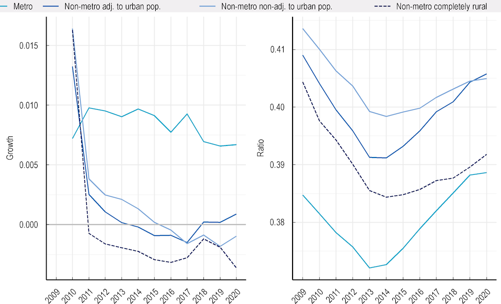
Source: U.S. Census Bureau (2022[7]), American Community Survey Data, https://www.census.gov/programs-surveys/acs/data.html.
There has been a long-running trend of declining labour participation (Kalleberg and Von Wachter, 2017[63]; Perez-Arce and Prados, 2021[64]). This was particularly pronounced in the aftermath of the 2008 financial crisis resulting in the trough in Figure 2.19 (right). Despite this trend, metro counties recovered and exceeded its pre-crisis worker level (as a share of the population), while non-metro AU counties recovered somewhat. By contrast, non-adjacent counties such as rural and non-metro NAU counties’ number of workers remained depressed. In rural counties, this was due to a decelerated loss of workers between 25 and 54 from 2013 onward.
Aging workers
The workforce in non-metropolitan counties is aging (Figure 2.20), in the United States and across OECD countries. Close to one-quarter of the population in non-metropolitan rural areas was over the age of 55 from 2006-10, while in the period of 2016-20, close to 29% of the population was over the age of 55. While the share of working age individuals below 24 remained the same in the two periods, the aging trend was primarily due to a loss of prime aged workers (25-54 years of age). While the workforce in the United States is aging as a whole, it is more pronounced in non-metropolitan regions and compounded by a lower share of primary workers. This trend is expected to continue (Martinez-Fernandez et al., 2012[65]), further aggravating pre-existing challenges in regional innovation. The aging trend of the non-metropolitan workforce would suggest a heightened need for life-long learning and upskilling programmes for non‑metropolitan regions (OECD, 2021[66]; OECD, 2022[67]).
Figure 2.20. Age-based demographic change
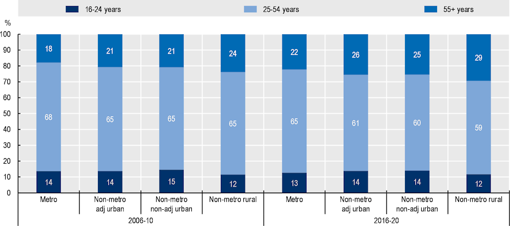
Note: Data are aggregated from county-level number of workers by age group.
Source: U.S. Census Bureau (2022[7]), American Community Survey Data, https://www.census.gov/programs-surveys/acs/data.html.
Gender diversity
Promoting gender diversity can inject new skills and opportunity into rural regions. Several studies have shown that gender diversity contributes positively to innovation and productivity (Gallego and Gutiérrez, 2018[68]; Reagans and Zuckerman, 2001[69]; Trax, Brunow and Suedekum, 2015[70]; Østergaard, Timmermans and Kristinsson, 2011[71]).26 In the United States, the Bureau of Labour Statistics found that 57.4% of women participated in the labour force, as compared to 69.2% of men, in 2019. However, this was still below its peak of 60% in 1999. Women also tended to cluster in educational and health services, financial services and hospitality, but were under-represented in key sectors of the non-metropolitan economy, such as the manufacturing and agricultural sectors (BLS, 2021[72]).
Challenges in equal pay and equal opportunities for employment and entrepreneurship are still prevalent in the United States and OECD countries (OECD, 2023[73]). Between 2016 and 2020, men were on average paid 31% more than women. While the gap is still substantial, it has decreased from close to 35% a decade earlier (between 2006 to 2010). This has mirrored improvements in the pay gap for women in several OECD countries (OECD, 2021[74]). A more recent finding, which focused only on full-time workers, found that while the average pay gap in OECD countries in 2021 was 12%, it remained higher than average in the US, at 17% (OECD, 2023[75]).27 Over the past half century, women have improved education attainment and become more active in higher paid occupations and sectors (BLS, 2021[72]; Blau and Kahn, 1994[76]; Fitzenberger, 2005[77]; Goos, Manning and Salomons, 2014[78]; Oostendorp, 2009[79]). However, the further away counties are from metropolitan regions, the more likely women are to continue to have stronger disparity with men’s wages (Figure 2.21). This finding has also been observed in many OECD countries (Murillo Huertas, Ramos and Simon, 2016[80]). Ensuring that innovation brings new activities to regions can create better opportunities and relieve monopsony power for women in small labour markets.
Figure 2.21. Gender wage gap
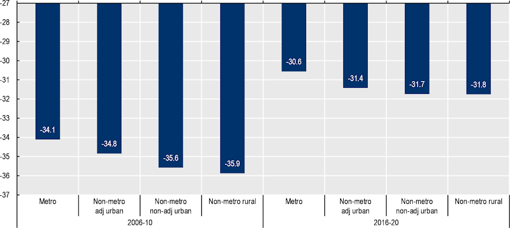
Note: Difference between median earnings of men and women relative to median earnings of men, weighted by population.
Source: U.S. Census Bureau (2022[7]), American Community Survey Data, https://www.census.gov/programs-surveys/acs/data.html.
Foreign-born workers
Migration is positively associated with innovation, entrepreneurship and firm performance across regions (OECD, 2022[81]; Kerr, 2018[82]; Guichard, Özgüzel and Kleine-Rueschkamp, forthcoming[83]). This is especially the case in federal countries like Switzerland and the United States (Beerli et al., 2021[84]; Breschi, 2016[85]; Hanson, Kerr and Turner, 2018[86]) — despite evidence of local labour market friction (OECD, 2022[81]). In the United States and other OECD countries like Canada, migration policies are actively being used to promote innovation (such as H1B visas in the US and the Canadian talent-based visa programme).
There is an increasing share of foreign workers on average across all United States counties (Figure 2.22). In part, if these are young foreign workers, it can offset the aging demographic in rural regions. However, in most rural counties, the share of foreign-born workers is much lower than other counties. It is also likely that metropolitan regions, which have a larger share of Higher Education and Research and Development (HERD) institutions, may be disproportionately benefiting from the innovative talents of high-skilled foreign-born workers, whereas the economic structure of rural counties, with a higher share of agriculture and manufacturing, may be more likely to experience higher demand for foreign-born workers with low skill levels or highly specialised skills.
Figure 2.22. Share of foreign-born workers
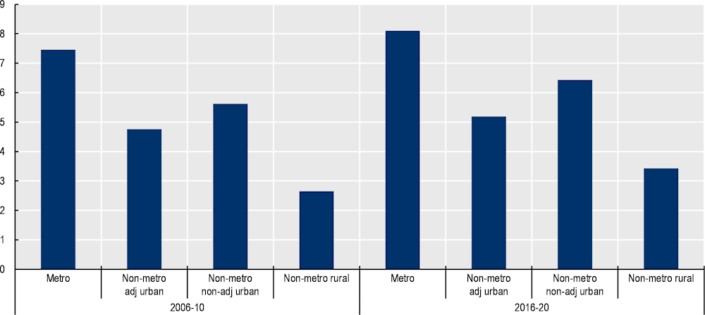
Note: Number of foreign-born workers are aggregated over territories then divided by total workers.
Source: U.S. Census Bureau (2022[7]), American Community Survey Data, https://www.census.gov/programs-surveys/acs/data.html.
Persistently poor counties
Promoting equity in access to opportunities for persistently poor across all places is a priority for the US administration. Under the EDA’s Equity investment priority, the question of reaching places that are persistently poor is a priority. Congressional guidance finds that a county is experiencing persistent poverty if poverty rates are currently at or above 20% and have been that high for the past 30 years. Using this definition, specific counties are designated as persistent poverty counties (PPCs). EDA’s equity investment priority finds that investment in PPCs is one way to meet the requirement of providing service to “underserved geographies.” Congress requires that EDA allocate at least 10% of its Public Works and Build-to-Scale appropriations to fund projects in PPCs (GAO, 2021[87]).
The share of counties that are considered persistently poor is five times higher in rural counties than metropolitan counties. While there are more persistently poor counties in metropolitan areas, 20% of counties in rural regions are considered persistently poor as compared to only 4% of metropolitan counties (Figure 2.23). The larger share of PPCs in metropolitan areas likely reflects the higher numbers of metropolitan counties (Table 2.1).
Figure 2.23. Shares of the population in persistently poor counties
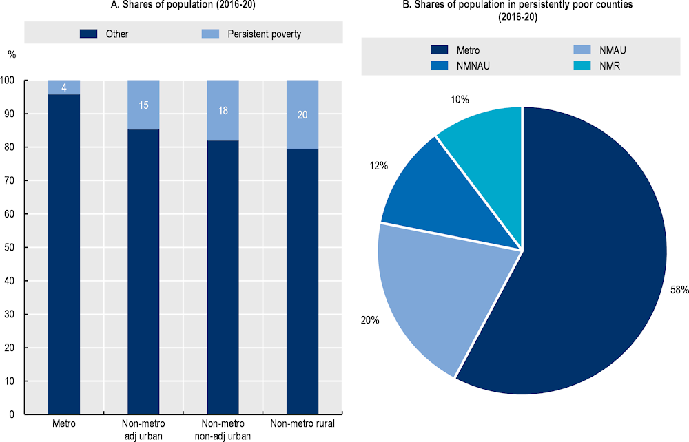
Note: Persistent poverty status is a county classification code used by the Economic Development Administration (EDA, 2021[88]). According to a congressional requirement, a county (or a county-level equivalent) is experiencing Persistent Poverty if their most recent poverty rate estimate, within the margin of error, equates to 20%, while also evidencing poverty rates of at least 20% in the 1990 and 2000 decennial censuses (i.e. 20% or greater poverty over the last 30 years). Specifically, for designation as a Persistent Poverty County (PPC), the county’s poverty rate must be 20% or greater (within the plus/minus range of the margin of error) of their most recent poverty estimates according to the U.S. Census Bureau’s Small Area Income and Poverty Estimates (SAIPE) dataset (https://www.census.gov/programs-surveys/saipe.html). The EDA uses the most recent SAIPE dataset (released December of every year, at which time the PPC list for that FY is updated). Metro refers to the counties classified as “Metropolitan.” NM-AU refers to the counties classified as “Non-metropolitan, adjacent to urban population.” NM-NAU refers to counties classified as “Non-metropolitan, non-adjacent to urban population.” NM-R refers to counties classified as “Non-metropolitan, completely rural.”
Source: U.S. Census Bureau (2022[7]), American Community Survey Data, https://www.census.gov/programs-surveys/acs/data.html.
Persistent poverty is associated with lower innovation outcomes across all types of counties. There is a strong difference in innovation outcomes across all counties, reinforcing the importance of socio-economic conditions to support innovation (Figure 2.24). Metropolitan counties tend to have high patenting intensity when they are not categorised as a persistently poor county; otherwise, their patenting intensity levels remain similar to those in persistently poor areas in non-metropolitan counties. Outcomes are similar for R&D investment across classification of counties, by persistent poverty status. The largest shares of investment in R&D are in counties that are not categorised as being in persistent poverty. Both patenting intensity and R&D investment are strongly associated with counties that do not face persistent poverty.
If benefits from innovation (for example, rents and wages) are reinvested in the community, innovation should be associated with a reduction in persistent poverty. However, as observed previously, some of the most innovative counties are not always the counties with the highest level of productivity suggesting that benefits of innovation may not always be local in nature. At the same time, a deep and entrenched lack of access to opportunities may also be causing a lower level of innovation. The fact that firms in counties may not be participating in R&D and patenting activities could be aggravating opportunities for persistently poor areas and directly contributing to sustaining people in high poverty levels over time.
Figure 2.24. Persistent poverty and innovation
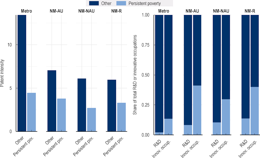
Note: Persistent poverty status is a county classification based on poverty statistics over the past 30 years (EDA, 2021[88]). Metro refers to the counties classified as “Metropolitan.” NM-AU refers to the counties classified as “Non-metropolitan, adjacent to urban population.” NM-NAU refers to counties classified as “Non-metropolitan, non-adjacent to urban population.” NM-R refers to counties classified as “Non-metropolitan, completely rural.” The x-axis labels on the right hand side refer to shares of total research and development funding, and shares of total innovative occupations.
Source: U.S. Census Bureau (2022[7]), American Community Survey Data, https://www.census.gov/programs-surveys/acs/data.html; BEA (2022[8]), Regional Economic Accounts, https://www.bea.gov/data/economic-accounts/regional; United States Patent and Trademark Office; Dotzel, K. and T. Wojan (2022[26]), “An occupational approach to analyzing regional invention”, https://ncses.nsf.gov/pubs/ncses22202.
Although the capacity for individuals to participate in high-tech innovation may be lower in non-metropolitan areas that are considered to be persistently poor, the relatively higher shares of innovative occupations as compared to R&D investment and relatively low levels of patent intensity in persistently poor areas suggest that the skills (in occupations) needed for high-tech innovation is still salient in non-metropolitan areas, despite the lack of innovation inputs (R&D investment) and outputs (patent intensity). It is important to recognise that in many non-metropolitan counties, there may be opportunities for innovative activities that are not being harnessed because of the lack of access to traditional innovation inputs and mechanisms to turn innovations into measurable outputs.
Innovation outcomes for non-metropolitan counties
In the next sub-sections, the regression and decomposition analyses reveal differences between counties focusing on differences between regions and their drivers. In this section, the regression analysis is a simple linear model that accounts for direct effects without controlling for interaction effects. In the following section, a full decomposition model estimates differences between metropolitan and non-metropolitan regions, including interaction effects.
There is a persistent and significant penalty for non-metropolitan regions in high-tech innovation. Column 2 of Table 2.2, demonstrates that belonging to a non-metropolitan county is associated with 1.34 fewer patents per 1 000 relevant workers as compared to metropolitan counties. In counties non-adjacent to urban counties, this impact is larger at 1.84 fewer patents per 1 000 relevant workers. However, completely rural counties are different than other types of counties. There is no statistically significant connection between being located in completely rural counties and patenting intensity. This seems to reinforce the fact that it is important to consider whether the indicator itself may be relevant to understanding innovation in remote rural counties.
The state contexts matter substantially for whether counties are likely to have high patent intensity. In Column 1 of Table 2.2, if we relax the effect of the state, we observe that there is no statistically significant difference between metropolitan and non-metropolitan counties. This suggests that state-level regulations are particularly important for determining high-tech innovation. In federal countries, like the United States, the role of the individual state is substantial in outcomes for individuals and firms. As described in the previous section much of the high-tech patenting activity is clustered on the coasts and in a few counties such as Santa Clarita and Los Angeles, both in California. Understanding how states with high patenting intensity operate can provide more evidence for states who may be looking to promote high patenting intensity, as one of the forms of innovation.
Despite the penalty on patent intensity, the penalty on productivity for non-metropolitan areas adjacent to metropolitan counties is non-existent, and relatively small in other types of counties. It is only when we account for state-level factors that there is a 3.4% decrease in productivity associated with non‑metropolitan counties. This is the case even when we control for sectoral, education and territorial (geographical) characteristics.28 In other words, state-level context impacts whether different geographies are disadvantaged when it comes to productivity. Without taking into consideration state-effects, there is no statistically significant difference between productivity in metropolitan counties and those in remote rural and non-metropolitan counties that are adjacent to metropolitan counties. The difference in outcomes as compared to metropolitan areas seem to suggest that counties close to urban areas may benefit from similar conditions as those in metropolitan areas no matter the state. This finding reinforces the importance of state-level conditions and functional areas that incorporate network effects when designing place-based policies for regional and rural innovation.
Lastly, while productivity as an indicator of innovation absorption suggests rural regions are benefiting from innovation absorption and innovating in different ways than metropolitan regions, there is still a penalty with regard to employment growth (Columns 3 and 4 of Table 2.2). The drop becomes more substantial in regions further away from urban areas, despite controlling from factors such as density and sector intensity. These findings can be impacted by policies on a state-level for non-metropolitan counties. In line with the findings from the macro-economic analysis in the first section, the loss in jobs is occurring in many different non-metropolitan counties, even though productivity and innovation absorption remain relatively high.
Table 2.2. Innovation outside of metropolitan areas
Territorial (geographical) impacts in county-level linear regressions (2006-10, 2011-15, 2016-20)
|
Metro and non-metro counties (RUCC, 2 categories) |
||||||
|---|---|---|---|---|---|---|
|
(1) |
(2) |
(3) |
(4) |
(5) |
(6) |
|
|
Patent intensity |
Employment (log) |
Labour productivity (log) |
||||
|
Non-metro |
-0.376 |
-1.341** |
-0.022*** |
-0.775*** |
-0.010 |
-0.034** |
|
[0.646] |
[0.565] |
[0.005] |
[0.036] |
[0.017] |
[0.016] |
|
|
Rural-urban county continuum (RUCC, 4 categories) |
||||||
|
(1) |
(2) |
(3) |
(4) |
(5) |
(6) |
|
|
Patent intensity |
Employment (log) |
Labour productivity (log) |
||||
|
Adjacent to urban |
-0.368 |
-1.491*** |
-0.020*** |
-0.473*** |
0.007 |
-0.028 |
|
[0.616] |
[0.566] |
[0.005] |
[0.038] |
[0.018] |
[0.018] |
|
|
Non-adjacent to urban |
-0.752 |
-1.839*** |
-0.024*** |
-0.859*** |
-0.038* |
-0.040** |
|
[0.810] |
[0.652] |
[0.006] |
[0.040] |
[0.022] |
[0.019] |
|
|
Rural |
1.428 |
-0.048 |
-0.038*** |
-1.378*** |
-0.042 |
-0.041* |
|
[1.211] |
[1.021] |
[0.008] |
[0.048] |
[0.029] |
[0.024] |
|
|
Observations |
5 876 |
5 876 |
6 274 |
6 274 |
6 171 |
6 171 |
|
Time FE |
Yes |
Yes |
Yes |
Yes |
Yes |
Yes |
|
Sector controls |
Yes |
Yes |
Yes |
Yes |
Yes |
Yes |
|
State demean |
No |
Yes |
No |
Yes |
No |
Yes |
|
Cluster |
County |
County |
County |
County |
County |
County |
Note: Patent intensity refers to patents per inventive occupation in thousands of workers in relevant occupations. Employment growth refers to log changes. Productivity is estimated as output (GDP) per worker. Because of confidentiality purposes, data used in this analysis is pooled across 5 years. There are three time periods in this regression, 2006-10, 2011-15 and 2016-20. All growth estimates are based on differences between each time period. All regression models are linear OLS regressions. All time-variant control variables are lagged from the previous year to reduce endogeneity. Other controls (including unreported controls) consist of year fixed effects, spending on Research and Development (log), the number of higher education and R&D institutions (log), the number of financial and bank service institutions (log) education shares, foreign born shares, migrant shares, oil county indicator, percentage of households with broadband, percentage of households with computers, average household income (logs), Gini index on household income, road length (log), density (log), share of migrants, total population, median age, work force age group shares, gender wage gap, median housing costs for owners as a percentage of income, median housing costs for renters as a percentage of income, and sector controls. Robust standard errors are in brackets. Errors are clustered on the county level. The second columns of each regression refer to regressions on variables that have been demeaned from state level averages. Statistical significance is defined as one of the following *** p<0.01, ** p<0.05, * p<0.1.
Source: U.S. Census Bureau (2022[7]), American Community Survey Data, https://www.census.gov/programs-surveys/acs/data.html; BEA (2022[8]), Regional Economic Accounts, https://www.bea.gov/data/economic-accounts/regional.
Drivers of high-tech innovation, employment and productivity
The following section uses data from the American Community Survey (ACS) and the Bureau of Economic Analysis on individual and firm characteristics. While household income, GDP and labour is available on a yearly basis, data from the ACS is often aggregated in 5-year intervals. For regression analysis, we use county level data for three time observations with year groupings of 2006-10, 2011-15, 2016-20. The BEA data is available on a county level on a yearly basis. We match ACS data with the BEA based on the last observable year. The panel is strongly balanced with 9 425 observations, 3 142 counties and three time observations (year groupings). The regression analysis starts with simple linear regressions, with demeaned state effects, and follows through using a decomposition model that compares outcomes for metropolitan and non-metropolitan areas, using the Oaxaca-Blinder model for estimating observable and unobservable differences in outcomes. It creates a counter factual exercise that helps us understand whether equal opportunity to the two types of territories (with available observables) can lead to a reduction in disparities. The model is further explained in Annex 2.D.
While we know that there is a penalty in high tech innovation, the findings are less detrimental on innovation absorption as measured by productivity for non-metropolitan regions. How can we understand what are driving these differences so that policies can better provide place-based support?29
Table 2.3. Differences in outcomes between metro and non-metropolitan counties
Oaxaca-Blinder Decomposition of Patent Intensity, Employment and Productivity, by Metro/Non-Metro counties
|
|
Metro |
Non-metro |
Total difference |
Explained |
Unexplained |
|||||
|---|---|---|---|---|---|---|---|---|---|---|
|
(1) Patent intensity |
9.539*** |
[0.732] |
6.860*** |
[0.466] |
2.679*** |
[0.630] |
0.832 |
[0.741] |
1.847* |
[1.012] |
|
(2) Employment (log) |
10.641*** |
[0.111] |
8.737*** |
[0.092] |
1.904*** |
[0.127] |
1.084*** |
[0.098] |
0.820*** |
[0.163] |
|
(3) Productivity (log) |
11.279*** |
[0.023] |
11.266*** |
[0.044] |
0.012 |
[0.033] |
-0.028 |
[0.038] |
0.041 |
[0.025] |
Note: The table above is a summary table for outcomes of the Oaxaca-Blinder decomposition, focusing on the difference between two groups, metro and non-metro. Patent intensity refers to patents per inventive occupation in thousands of workers in relevant occupations. Employment growth refers to log changes. Productivity is estimated as output (GDP) per worker. Because of confidentiality purposes, data used in this analysis is pooled across five years. There are three time periods in this regression, 2006-10, 2011-15 and 2016-20. All growth estimates are based on differences between these time periods. All regression models are linear OLS regressions. All time-variant control variables are lagged from the previous year to reduce endogeneity. Other controls including those unreported consist of year fixed effects, spending on Research and Development (log), the number of higher education and R&D institutions (log), the number of financial and bank service institutions (log) education shares, foreign born shares, migrant shares, oil county indicator, percentage of households with broadband, percentage of households with computers, average household income (logs), Gini index on household income, road length (log), density (log), share of migrants, total population, median age, work force age group shares, gender wage gap, median housing costs for owners as a percentage of income, median housing costs for renters as a percentage of income, and sector controls. Robust standard errors are in brackets. Errors are clustered on the county level. Only state demeaned results are reported. Statistical significance is defined as one of the following *** p<0.01, ** p<0.05, * p<0.1.
Source: U.S. Census Bureau (2022[7]), American Community Survey Data, https://www.census.gov/programs-surveys/acs/data.html; BEA (2022[8]), Regional Economic Accounts, https://www.bea.gov/data/economic-accounts/regional.
There are 2.7 more patents per inventive occupation in the United States in metropolitan counties than in non-metropolitan counties and there is close to a two-fold increase in employment growth in metropolitan counties as compared to non-metropolitan counties (Table 2.3). These findings hold despite direct and interaction effects of the sectoral, educational, and socio-economic attributes of counties as described in the note of Table 2.3.30 Furthermore, as discussed before in the chapter, patent intensities are highly sensitive to the inclusion of state-level effects, meaning that they may highly be contingent on state level regulation and opportunities.
Density and distance are associated with patent intensity, but results are mixed between metropolitan and non-metropolitan counties. For example, less density is associated with patent intensity in metropolitan areas but not non-metropolitan areas (Annex Table 2.E.1).31 In metropolitan areas, a 10% increase in the density of your county is associated with 1.2 less patents per inventive occupation. This is not the case in non-metropolitan counties, where the relationship is not statistically significant. However, one of the strongest indicators of patent intensity in non-metropolitan regions is physical infrastructure (road length). A 10% increase in road length is associated with 4.4 fewer patents per person (with a relevant occupation) in non-metropolitan counties. The larger the size (road distance) within the county, regardless of the density of the population, the less likely they are to file a patent. In metropolitan counties, the results are not statistically significant. Lastly, a high average household income is positively associated with patent intensity. A 10% increase in average household incomes is associated with 18 more patents per person (in relevant occupations). The magnitude of this variable is large, but likely associated with the occupation of the main household earner.32
With equal socio-economic opportunities across territories, there is no statistically significant difference between productivity – our proxy for the capacity to adopt innovation – between counties (row 3 of Table 2.3). This is the case regardless of the state counties are located in. The fact that productivity does not follow the same territorial (geographical) trend as patent intensity is substantial. In addition, the decomposition results for patent intensity are sensitive to whether or not we are controlling for the state where counties are located. The fact that this is not the case with productivity suggests that this may be a more comparable statistic to use as a measure of innovation, both because of its statistical features that are applicable across sectors, and because it is less reliant on state-level effects.
What can we say about drivers of productivity in non-metropolitan regions? Some of the standard measures of innovation such as the number of Higher Education and Research and Development (HERD) institutions and R&D spending have no impact on productivity in non-metropolitan regions.
While an increase in the number of HERD institutions is associated with a 1.6% increase in productivity in metropolitan regions, it does not drive productivity in non-metropolitan regions (columns 5 and 6 of Annex Table 2.E.1). At the same time, the share of HERD institutions is positively associated with patent intensity in metropolitan counties, but negatively associated with patent intensity in non-metropolitan counties. On the other hand, the share of college educated students is associated positively with productivity in non‑metropolitan counties yet negatively in metropolitan counties. While non-statistically-significant, it seems to suggest that investing in education in non-metropolitan regions is still positively associated with productivity, but not necessarily high-tech innovation (patent intensity) in non-metropolitan areas. Further research on the role of specific types of universities with stronger ties to the rural counties, such as Land Grant Colleges, finds a statistically positive association between universities and ingenuity among engineers (Maloney and Valencia Caicedo, 2022[89]). However, other studies find that land grant universities were an important determinant of local-based innovation (Lyons, Miller and Mann, 2018[90]).
Critically, the role of building human capital for innovation is important. For example, better management practices are often associated with better outcomes for firms in terms of productivity and employment (Bloom and Van Reenen, 2007[91]). Yet, rural entrepreneurs are often likely to start companies without prior training, or access to similar socio-economic resources as those in rural areas (OECD, 2022[6]). Many governments try to address this challenge through provision of entrepreneurial courses; however, sometimes programmes to encourage better entrepreneurial skills have no direct effect on innovation outcomes. How programmes for developing human capital are targeted is important, and building on the pre-existing desires and opportunities for entrepreneurs to start a new endeavour during early school years (primary school) is critical (Jardim, Bártolo and Pinho, 2021[92]), as is further discussed in Chapter 4. Such programmes when targeted to young individuals had positive impacts on entrepreneurial skills, creativity, self-confidence, power of argument, and construction of social skills in relationships and interpersonal and groups settings.
Increased spending on research and development (R&D) for innovation is associated with a 4.1% decline in jobs in the following year in metropolitan areas, but a 19.4% increase in jobs in the following year for non-metropolitan areas (Annex Table 2.E.1). This finding is similar for in non-metropolitan areas of Switzerland (OECD, 2022[3]). R&D investments outside of metropolitan areas are associated with job growth, while they are associated with job retraction in metropolitan regions. This increase in jobs however is not simultaneously associated with productivity in metropolitan regions or non-metropolitan regions.
Finally, a few characteristics that the current model considers will be further developed in the following chapters of the report. This includes access to finance (Chapter 3). In general, there is a positive association between financial institutions, employment growth and productivity in metropolitan counties, but not in non-metropolitan counties. This could imply that financial institutions alone may not be enough to increase access to finance and innovation, in particular when financial markets are not functioning effectively, and when quick-wins are favoured over slower innovation (James, Kotak and Tsomocos, 2022[93]).
When it comes to broadband (Chapter 4), increasing the percentage of households with access to broadband is positively associated with employment growth in metropolitan counties, but not in non‑metropolitan counties. This may suggest that broadband alone, without a focus on quality or affordability may not have the same impact in non-metropolitan counties as it does in metropolitan counties.
Lastly, college-educated populations are positively associated with employment growth in metropolitan areas, but not in non-metropolitan counties. In the context of non-metropolitan counties, this may indicate a difference in the demand for different skilled workers. Anecdotal evidence suggests that rural and non‑metropolitan regions may need more support for vocational training and quality education in primary and secondary schools before benefiting from highly educated workers as in metropolitan regions. The subject will be further explored in Chapter 4.
Annex 2.A. Defining rural geographies
The definition of “rural” adopted for this report is based on the United States Department of Agriculture (USDA)’s classification that distinguishes between rural and urban counties, known as the Rural-Urban Continuum Codes (RUCC). The RUCC is built on the metropolitan and non-metropolitan dichotomy determined by the Office of Management and Budget. USDA then further refined the binary grouping to create a continuum of three metro and six non-metro sub-groups, resulting in a nine-group county classification. While the latest revision occurred in 2013, the classification originally dates back to 1975 at its first release, and is updated every 10 years after the release of the decennial census data.
For non-metropolitan regions, proximity and connectiveness to an urban region is an important predictor of growth (OECD, 2016[94]). Because of the importance of connectedness between places for innovation, the analysis in the chapter takes the approach of grouping non-metropolitan countries by adjacency. Taking the functional area approach may encourage networking and linkages across territories. Furthermore, this could have an implication on the scale of interventions (see Chapter 3) and whether territories have access to additional federal resources (CORI, 2022[95]).
Therefore, the nine original RUCC groupings have been reduced to four: metropolitan counties (MR), non-metropolitan regions adjacent to metropolitan counties (AU), non-metropolitan counties not adjacent to metropolitan counties (NAU), and remote non-metropolitan counties (rural).
To explain, this includes namely two combinations based on adjacency of different types of non-metro, non-rural counties. First, it includes the combination of non-metro counties with an urban population of 20 000 or more, that are adjacent to a metro area (RUCC 4), with non-metro counties with an urban population of 2 500 to 19 999, adjacent to a metro area (RUCC 6) to create a simplified category of non‑metropolitan adjacent to urban areas (Non-metro AU). Secondly, it includes the combination of non‑metro counties with urban population of 20 000 or more, not adjacent to a metro area (RUCC 5), with non-metro counties urban population of 2 500 to 19 999, not adjacent to a metro area (RUCC 7). Finally, it includes the combination of both rural categories that have less than 2 500 urban populations.
As such, the reduced classification, focusing on proximity as a unifying factor, has the goal of shifting emphasis from the size of non-metropolitan regions to their relationship to urban centres. Additionally, it has the advantage of minimising category change due to population movement across the 2010 decade where analysis of this chapter is based. The reclassification is illustrated in Annex Table 2.A.1. This is most notable for non-metropolitan regions, which are interconnected with and shaped by their urban neighbours, while remaining distinct entities in terms of their economic functions, settlement patterns and ways of life. By contrast, in remote rural places there are fewer direct connections with cities so local residents and firms must rely almost exclusively on local providers of goods and services. The reduced classification attempts to capture and account for these dynamics.
Annex Figure 2.A.1. US counties by simplified USDA Rural-Urban Continuum Classification
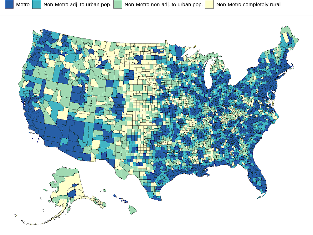
Source: Based on USDA (2013[5]), Rural-Urban Continuum Codes, https://www.ers.usda.gov/data-products/rural-urban-continuum-codes.
Annex Table 2.A.1. Simplified classification of 2013 RUCC by adjacency status
|
2013 RUCC code |
2013 RUCC description |
OECD simplification |
OECD simplification, in-text short hand |
|---|---|---|---|
|
1 |
Counties in metro areas of 1 million population or more |
Metro |
Metro |
|
2 |
Counties in metro areas of 250 000 to 1 million population |
||
|
3 |
Counties in metro areas of fewer than 250 000 population |
||
|
4 |
Urban population of 20 000 or more, adjacent to a metro area |
Non-Metro adjacent to urban population |
Non-metro AU |
|
6 |
Urban population of 2 500 to 19 999, adjacent to a metro area |
||
|
5 |
Urban population of 20 000 or more, not adjacent to a metro area |
Non-Metro not adjacent to urban population |
Non-metro NAU |
|
7 |
Urban population of 2 500 to 19 999, not adjacent to a metro area |
||
|
8 |
Completely rural or less than 2 500 urban population, adjacent to a metro area |
Non-metro completely rural |
Rural |
|
9 |
Completely rural or less than 2 500 urban population, not adjacent to a metro area |
Source: Based on USDA (2013[5]), Rural-Urban Continuum Codes, https://www.ers.usda.gov/data-products/rural-urban-continuum-codes.
Annex Box 2.A.1. Description of OECD classifications for places and US sectors
OECD classification of rural regions: Defining rural using physical and driving distances within administrative boundaries
The most recent definitions of rural regions have benefited from a reflection on the combination of physical (“first-nature”) and human (“second-nature”) geographies. Rural regions are defined by economic remoteness, with three distinct features related to the physical distance to major markets, economic connectedness, and sector specialisation. Considering these features, rural regions are physically distant to major markets, with specialisation in niche markets and those linked with natural resources such as agriculture and tourism. The degree of economic connectedness with surrounding areas may vary by relative density, infrastructure availability and complementarities between and within rural regions.
In consultation with OECD national governments, the OECD harmonised a set of guidelines for classifying geographical characteristics across countries that avoid the traditional, and sometimes harmful, rural-urban dichotomy. This unified definition of “rural” provides the basis for analysis across countries within rural economies (OECD, 2020[96]). The OECD classified large and small regions within each country, and drew on characteristics of functional urban area within small regions in each country. Each country’s large region, referred to as Territorial Level 2 (TL2), and small region Territorial Level 3 (TL3) are based on administrative zones. In the United States, the Territorial Level 2 (TL2) refers to the 51 states and the District of Columbia, while TL3 refers to 179 economic areas new classification based on functional urban areas (FUA) incorporates density and the driving estimations for the time it takes to access dense metropolitan areas for each TL3 region. To the furthest extent possible, non-metropolitan regions are defined as one of three types of small administrative regions (TL 3) with less than 50% of the regional population living in metropolitan areas.
Non-metropolitan regions are defined as having less than 50% of the population living in a functional urban area with a population larger than 250K. The 3 types of non-metropolitan county include:
Non-metropolitan regions with access to a metropolitan region: These regions have 50% or more of the regional population that lives within a 60-minute drive of a metropolitan area. This is similar in part to towns and suburbs surrounding the distant periphery of major metropolitan centres. An example of such regions includes Tyrolean Oberland in Austria (AT334), Montmagny in Quebec, Canada (CA2418), Jura in France (FRC22), or Nagasaki in Japan (JPJ42). The challenges of such regions often are tied to economies of metropolitan areas, while focusing on industries such as tourism, without some of the infrastructure barriers of less densely populated areas.
Non-metropolitan regions with access to small- or medium-sized cities: These regions are regions with 50% or more of the regional population living within a 60-minute drive from a small- or medium-sized city. Examples of these types of regions include the administrative district of Neufchâteau in Belgium (BE344), San Antonio in Chile (CL056), South Bohemia in the Czech Republic (CZ031), East Lancashire in the United Kingdom (UKD46) or Springfield in Illinois, the United States (US158). These regions have a strong manufacturing base and linkages to neighbouring economies.
Non-metropolitan remote regions: These regions have 50% or more of the regional population without access to a functional urban area within a 60-minute drive. Examples of these types of regions include Capital Region, New South Wales in Australia (AU101), La Côte‑de-Gaspé, Quebec in Canada (CA2403), Orkney Islands, Scotland in the United Kingdom (UKM65), and Anchorage, Arkansas in the United States (US008). The schematic breakdown is available in the figure below.
Annex Figure 2.A.2. OECD typology for access to cities
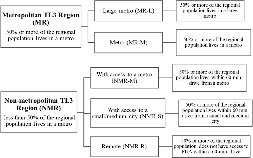
Note: Large metro: functional urban area with a population larger than 1.5 million; Metro: functional urban area with population larger than 250 000; small or medium city: functional urban areas with population smaller or equal to 250 000.
Source: OECD (2020[96]), Rural Well-being: Geography of Opportunities, https://doi.org/10.1787/d25cef80-en; Fadic, M. et al. (2019[9]), “Classifying small (TL3) regions based on metropolitan population, low density and remoteness”, https://doi.org/10.1787/b902cc00-en.
Sector classifications
The industrial sector classification used in this report follows the one provided by the government agencies where the data originate, which is mainly the North American Industry Classification System. These industrial groupings are used in the American Community Survey from the U.S. Census Bureau and is the basis for sectoral analysis of this chapter. Abbreviations may be used for brevity.
Extraction dependent counties
Due to supra-national oil and gas price fluctuations and the volatility of output based on global trends rather than firm production processes, the inclusion of oil and gas industries in analysis on drivers of innovation and productivity can be misleading. Because of the outlier effects exerted by counties with a high share of employment in oil and gas extraction, when necessary, such counties are excluded from analysis in this chapter. The list of such counties is obtained from the U.S. Bureau of Labor Statistics (2021[16]) based on employment concentration of the oil and gas sector in June 2014. Where of interest, results including these counties are reported separately, or controlled for using a binary indicator.
Annex Table 2.A.2. Sector classifications
|
NAICS 2017 classification |
Industrial sector |
Abbreviation used in the chapter |
|---|---|---|
|
11, 21 |
Agriculture, forestry, fishing and hunting, and mining |
Agriculture |
|
71, 72 |
Arts, entertainment, and recreation, and accommodation and food services |
Recreation |
|
23 |
Construction |
Construction |
|
61, 62 |
Educational services, and health care and social assistance |
Education and social services |
|
52, 53 |
Finance and insurance, and real estate and rental and leasing |
Finance, insurance, and real estate |
|
51 |
Information |
Information |
|
31-33 |
Manufacturing |
Manufacturing |
|
81 |
Other services, except public administration |
Other services (non-public) |
|
54, 55, 56 |
Professional, scientific, and management, and administrative and waste management service |
Professional services |
|
44, 45 |
Retail trade |
Retail trade |
|
48, 49, 22 |
Transportation and warehousing, and utilities |
Transportation and utilities |
|
42 |
Wholesale trade |
Wholesale trade |
Source: US Census Bureau (n.d.[97]), North American Industry Classification System – NAICS, https://www.census.gov/naics/?58967?yearbck=2017.
Annex 2.B. Rural proofing innovation
The way we understand and define innovation matters (OECD, 2022[6]). The OECD has fostered, since the 1990s, a common approach to measure and report statistics on innovations. This approach is contained in the Oslo Manual, a document produced by the OECD Working Party of National Experts on Science and Technology Indicators (NESTI) that has been adopted by over 80 countries. According to the 4th revision of the Oslo Manual, innovation can be defined as “a new or improved product or process (or combination thereof) that differs significantly from the unit’s previous products or processes and that has been made available to potential users (product) or brought into use by the unit (process)” (OECD/Eurostat, 2018[35]). The distinction between innovation as an outcome (an innovation) and the activities by which innovations come about (innovation activities) is an important one.
Other major additions to the previous versions include measuring innovation not only from businesses but also other organisations and individuals; updates to improve harmonisation between core definitions and taxation; better accounting of globalisation, digitalisation, and trends in investment in intangible assets; guidance on measuring internal and external factors influencing business innovation; prioritisation of the measurements of government policies on innovation; expansion of methodological guidelines; guidance on the use of innovation data and a new glossary.
Furthermore, the recent revision of the manual now includes definitions specifically for the business sector that target product and process innovations, including management practices, that had not been introduced to the market previously or brought to use by the firm, as well as innovation related activities that include developmental, financial and commercial activities intending to result in an innovation.
The literature on measures of innovation has been largely focused on patent production. This more conventional metric is often better suited for product innovations in large firms that specialise in the manufacturing- or R&D-intensive sectors and depend on heavier capital and resource expenditures. However, a larger share of firms in rural regions are often small, and dedicated to the service or natural resource sectors (Freshwater et al., 2019[40]), where innovation is incremental or is characterised by a strong use of social and human capital (Shearmur, Carrincazeaux and Doloreux, 2016[98]). Indeed, Mann and Loveridge (2020[99]) report that patent applications may be a less useful proxy for innovation by rural firms than for urban firms. Annex 2.C gives an overview of this discussion.
Annex 2.C. Patentable occupations
The proposal on adjusting innovation indicators for the occupational structure or rural economies comes from discussions within the OECD Expert Advisory Committee for Rural Innovation. During the sessions, several rural academics identified structural problems associated with how innovation is measured in rural areas, and why the bias associated may not be geographically homogenous. To address this, work by Dotzel (2017[100]) and Wojan (2021[101]) proposes an occupation-driven approach for analysing regional invention. The authors argue that patenting rates should be computed on the subset of workers that might plausibly contribute to patenting. To do this, the authors regress the aggregate number of patents produced in commuting zone during the period 2000-05 on the share of the workforce employed in a selection of detailed census occupations. The authors’ commuting zone-level regression includes controls on the patent stock, human capital share (working age population with a bachelor’s degree or higher), population density, a natural amenity score, and the wage-rental ratio. They apply the analysis on a core set of occupations (from the U.S. Department of Labor’s Employment and Training Administration’s O*NET’s database) defined by the National Science Foundation’s classification of science, engineering and technical (SET) occupations, along with an iterative random selection of other occupations that may have a strong association with patenting. Ten thousand regressions are estimated with 19 non-SET occupations randomly included in each estimation. The inventive subset inclusion criteria for the non-SET occupations are those occupations associated with coefficients that are positive and significant in at least 75% of their regressions in the metro or non-metro analysis. Of the 300 non-SET occupations included in the analysis, 11 are identified as inventive, that is, consistently associated with positive, significant coefficients.
Annex Table 2.C.1 below provides a list of occupations with a relatively high probability to patent. Furthermore, Annex Figure 2.C.1 and Annex Table 2.C.1 demonstrate the distribution of these occupations as a share of total employed population (patent intensity) across the United States. Adjusting for these shares reduce disparities in patenting intensities between territories.
Annex Table 2.C.1. Inventive occupations
Occupations with a high (>75%) probability to patent
|
Census Code(s) |
Occupation |
|---|---|
|
100-176, 190-196 |
Science, engineering, and technical (SET) occupations |
|
005 |
Marketing and sales managers |
|
030 |
Engineering managers |
|
181 |
Market and survey researchers |
|
263 |
Designers |
|
284 |
Technical writers |
|
772 |
Electrical, electronics, and electromechanical assemblers |
|
790 |
Computer control programmers and operators |
|
803 |
Machinists |
|
806 |
Model makers and patternmakers, metal and plastic |
|
813 |
Tool and die makers |
|
884 |
Semiconductor processors |
Note: Occupations associated with coefficients that are positive and significant in at least 75% of their regressions in the metro or non-metro analysis are characterised as inventive.
Source: Dotzel, K. (2017[100]), “Three essays on human capital and innovation in the United States”, http://orcid.org/0000-0002-3363-8751; Wojan, T. (2021[101]), An Occupational Approach for Analyzing Regional Invention, https://ncses.nsf.gov/pubs/ncses22202.
Annex Figure 2.C.1. Inventive occupations in the United States
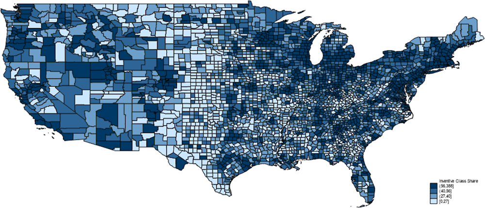
Note: Shares represent the shares of occupations likely to patent as a part of all employed labour defined in Wojan (2021[101]).
Source: US Census Bureau.
Annex 2.D. Education and patent intensity
While higher education and research and development (HERD) institutions are often associated with high levels of innovation, there seems to be a non-linear correlation with patent intensity across territories. HERD is positively associated with patent intensities in metropolitan regions, but this not as clear in rural counties where the counties with the lowest shares of HERD institutions have the highest average patent intensity (Annex Figure 2.D.1). It suggests that innovation may occur differently in rural counties, and that patent intensity may be tied to other characteristics.
Annex Figure 2.D.1. HERD and patent intensity
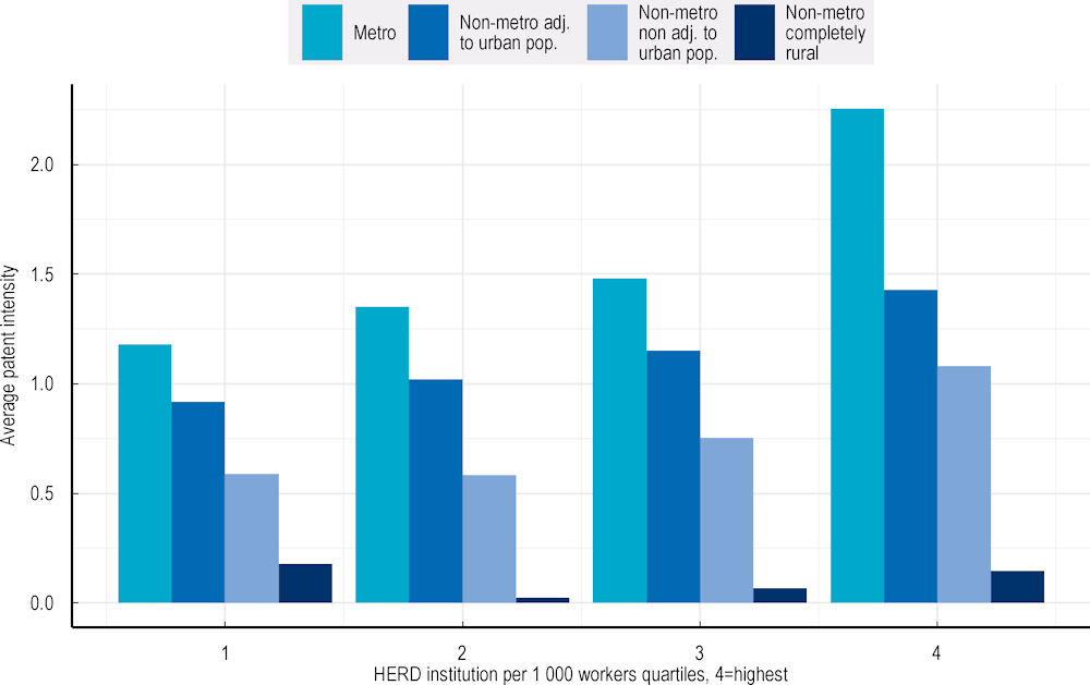
Note: Counties have been ranked by their position and the distribution of HERD institutions per 1 000 workers across the United States. The bars indicate the average patent intensity by county class within their respective quartile.
Source: U.S. Census Bureau (2022[7]), American Community Survey Data, https://www.census.gov/programs-surveys/acs/data.html; County Business Patterns Data, https://www.census.gov/programs-surveys/cbp/data.html ; United States Patent and Trademark Office; National Science Foundation; Dotzel, K. and T. Wojan (2022[26]), “An occupational approach to analyzing regional invention”, https://ncses.nsf.gov/pubs/ncses22202 (accessed on 15 July 2022).
Annex 2.E. Understanding explained and unexplained differences between two groups through a counter-factual exercise: The Oaxaca‑Blinder Decomposition
In the early 1970s, Roland Oaxaca and Blinder popularised a framework for decomposing differences between two groups attributed to observables and non-observables. A typical application of the model is the creation of a counter-factual that divides any observed gap between two exclusive sub-groups into components that are observed as characteristics of individuals, and a component that contributes to a difference in the structure of outcome variables (Fortin, Lemieux and Firpo, 2011[102]). Since then, the Oaxaca-Blinder decomposition has been one of the most widely used models for understanding what may be attributed to observable and non-observable characteristics between two groups. A simplified version of their model decomposes intergroup differences in two parts. The decomposition aims to understand what part of the differences in the mean outcomes of each group: where Y is expected outcome variables for group A and B.
We can apply a linear estimation form and model assumptions to the differences between both groups and generate the following for our reference groups A and B:
which gives us three components. The first component is the difference between observable predictors (“endowments”). The second part is the difference between coefficients (“coefficients effect”). The last component is the interaction effect, which is the difference simultaneously attributed between the two groups. The coefficients effect is the outcome that measures the expected change in group B’s mean outcome if group B had group A’s coefficients. If we applied this to male-female wage gaps, the coefficient effect would measure the mean outcome of women, if women had the same attributes as men. The second and third part of the decomposition are often referred to as the unexplained differences between groups. Most applications of this method have been used to look at differences in gender wage gap, but has also been used for differences between ethnic, union membership and immigrant status in the labour economics literature. It has also been extended to analysis in gaps in test scores, schools and countries. The decomposition has some similar attributes to the programme evaluation literature, as it generates counter-factual interpretation through the assignment of a “treatment” as the unobservable component of the decomposition, but falls short of fully understanding the mechanisms under which discrimination, or unobserved differences, occur (Fortin, Lemieux and Firpo, 2011[102]; Jann, 2008[103]; Oaxaca, 1973[104]).
The results of the exercise applied to metro and non-metro areas are included in the text of this chapter, and the extended results are provided in Annex Table 2.E.1 below.
Annex Table 2.E.1. Oaxaca-Blinder Decompositions by Classification of counties
County-level linear regressions (2006-10, 2011-15, 2016-20)
|
|
(1) |
(2) |
(3) |
(4) |
(5) |
(6) |
|---|---|---|---|---|---|---|
|
Patent intensity |
Employment (log) |
Productivity (log) |
||||
|
Metro |
Non-metro |
Metro |
Non-metro |
Metro |
Non-metro |
|
|
R&D Spending |
-0.232 |
0.401 |
-0.042*** |
0.200*** |
-0.003 |
0.009 |
|
[0.400] |
[0.383] |
[0.013] |
[0.070] |
[0.008] |
[0.013] |
|
|
Higher Education R&D institutions (log) |
0.171 |
-0.714 |
0.005 |
-0.236*** |
0.016*** |
-0.023 |
|
[0.401] |
[0.484] |
[0.007] |
[0.088] |
[0.004] |
[0.015] |
|
|
Secondary Education (share) |
0.064 |
0.051 |
0.008 |
0.004 |
0.006 |
-0.003 |
|
[0.193] |
[0.140] |
[0.007] |
[0.011] |
[0.006] |
[0.004] |
|
|
College Education (share) |
0.297 |
-0.403 |
0.098*** |
-0.013 |
-0.076 |
0.026 |
|
[0.730] |
[0.552] |
[0.023] |
[0.044] |
[0.049] |
[0.024] |
|
|
Doctoral Education (share) |
0.290 |
0.015 |
-0.003 |
-0.001 |
-0.001 |
0.001 |
|
[0.326] |
[0.211] |
[0.007] |
[0.009] |
[0.003] |
[0.003] |
|
|
Households with Broadband (%) |
0.460 |
0.478 |
0.033** |
0.040 |
-0.001 |
0.010 |
|
[0.714] |
[0.471] |
[0.017] |
[0.029] |
[0.013] |
[0.013] |
|
|
Financial Inst (log) |
0.174 |
-0.324 |
0.026* |
-0.064* |
-0.013 |
-0.016 |
|
[0.480] |
[0.377] |
[0.014] |
[0.035] |
[0.014] |
[0.013] |
|
|
Road Length (log) |
0.890 |
-0.175 |
0.102** |
0.074 |
0.107** |
0.006 |
|
[1.411] |
[1.162] |
[0.044] |
[0.046] |
[0.049] |
[0.024] |
|
|
Density, sqm (log) |
0.279 |
-0.441** |
0.033*** |
-0.026 |
0.039 |
-0.025** |
|
[0.287] |
[0.223] |
[0.012] |
[0.018] |
[0.025] |
[0.010] |
|
|
Migrants (%) |
-0.126** |
-0.048 |
0.004** |
-0.091*** |
0.002 |
-0.003 |
|
[0.061] |
[0.186] |
[0.002] |
[0.034] |
[0.002] |
[0.004] |
|
|
Household average income (log) |
0.016 |
-0.008 |
-0.001 |
0.001 |
-0.001 |
0.001 |
|
[0.015] |
[0.010] |
[0.001] |
[0.001] |
[0.001] |
[0.001] |
|
|
Gini Indicator |
-0.154 |
0.024 |
-0.014*** |
0.012*** |
0.008 |
-0.003* |
|
[0.182] |
[0.078] |
[0.005] |
[0.004] |
[0.005] |
[0.002] |
|
|
Population (log) |
0.130 |
0.006 |
0.000 |
-0.001 |
0.001 |
-0.001 |
|
[0.098] |
[0.027] |
[0.001] |
[0.002] |
[0.001] |
[0.001] |
|
|
Young Workforce (16-24, %) |
1.814*** |
0.296 |
-0.158*** |
0.036 |
0.179** |
-0.007 |
|
[0.666] |
[0.271] |
[0.046] |
[0.026] |
[0.070] |
[0.018] |
|
|
Prime age Workforce (25-54, %) |
-0.285* |
0.058 |
0.002 |
0.004* |
-0.004* |
0.003** |
|
[0.154] |
[0.046] |
[0.003] |
[0.002] |
[0.002] |
[0.001] |
|
|
Median housing costs (own, % inc) |
-3.303 |
0.933 |
1.012*** |
-0.008 |
-0.248* |
0.040 |
|
[2.238] |
[1.623] |
[0.110] |
[0.078] |
[0.149] |
[0.056] |
|
|
Median housing costs (rent, % inc) |
-0.906 |
-0.458 |
0.014 |
-0.031 |
0.060 |
-0.019 |
|
[0.710] |
[0.292] |
[0.021] |
[0.024] |
[0.037] |
[0.014] |
|
|
Observations |
2 938 |
2 938 |
3 138 |
3 138 |
3 087 |
3 087 |
Note: The table above is a summary table for outcomes of the Oaxaca-Blinder decomposition, focusing on the difference between two groups, metro and non-metro. Patent intensity refers to patents per inventive occupation in thousands of workers in relevant occupations. Employment growth refers to log changes. Productivity is estimated as output (GDP) per worker. Because of confidentiality purposes, data used in this analysis is pooled across five years. There are three time periods in this regression, 2006-10, 2011-15 and 2016-20. All growth estimates are based on differences between these time periods. All regression models are linear OLS regressions. All time-variant control variables are lagged from the previous year to reduce endogeneity. Other controls (including those that are unreported) consist of year fixed effects, spending on Research and Development (log), the number of higher education and R&D institutions (log), the number of financial and bank service institutions (log) education shares, foreign born shares, migrant shares, oil county indicator, percentage of households with broadband, percentage of households with computers, average household income (logs), Gini index on household income, road length (log), density (log), share of migrants, total population, median age, work force age group shares, gender wage gap, median housing costs for owners as a percentage of income, median housing costs for renters as a percentage of income, and sector controls. Robust standard errors are in brackets. Errors are clustered on the county level. Only state demeaned results are reported. Statistical significance is defined as one of the following *** p<0.01, ** p<0.05, * p<0.1.
Source: U.S. Census Bureau (2022[7]), American Community Survey Data, https://www.census.gov/programs-surveys/acs/data.html; BEA (2022[8]), Regional Economic Accounts, https://www.bea.gov/data/economic-accounts/regional.
References
[51] Aghion, P. et al. (2018), “Innovation and top income inequality”, The Review of Economic Studies, Vol. 86/1, pp. 1-45, https://doi.org/10.1093/restud/rdy027.
[37] Aghion, P. et al. (2001), “Competition, imitation and growth with step-by-step innovation”, Review of Economic Studies, Vol. 68/3, pp. 467-492, https://doi.org/10.1111/1467-937x.00177.
[105] Ahlfeldt, G. and E. Pietrostefani (2017), The Economic Effects of Density: A Synthesis.
[30] Akçomak, İ. and B. ter Weel (2009), “Social capital, innovation and growth: Evidence from Europe”, European Economic Review, Vol. 53/5, pp. 544-567, https://doi.org/10.1016/j.euroecorev.2008.10.001.
[38] Andersson, F. et al. (2009), “Reaching for the stars: Who pays for talent in innovative industries?”, The Economic Journal, Vol. 119/538, pp. F308-F332, https://doi.org/10.1111/j.1468-0297.2009.02277.x.
[15] Andrews, D., C. Criscuolo and P. Gal (2016), “The Best versus the Rest: The Global Productivity Slowdown, Divergence across Firms and the Role of Public Policy”, OECD Productivity Working Papers, No. 5, OECD Publishing, Paris, https://doi.org/10.1787/63629cc9-en (accessed on 27 July 2022).
[14] Angel, S. and A. Blei (2016), “The productivity of American cities: How densification, relocation, and greater mobility sustain the productive advantage of larger U.S. metropolitan labor markets”, Cities, Vol. 51, pp. 36-51, https://doi.org/10.1016/J.CITIES.2015.11.030.
[8] BEA (2022), Regional Economic Accounts, United States Bureau of Economic Analysis, https://www.bea.gov/data/economic-accounts/regional (accessed on 29 July 2022).
[12] BEA (2017), “Gross Domestic Product, 4th quarter and annual 2016 (third estimate); Corporate Profits, 4th quarter and annual 2016”, United States Bureau of Economic Analysis, https://www.bea.gov/news/2017/gross-domestic-product-4th-quarter-and-annual-2016-third-estimate-corporate-profits-4th (accessed on 13 July 2022).
[84] Beerli, A. et al. (2021), “The abolition of immigration restrictions and the performance of firms and workers: Evidence from Switzerland”, American Economic Review, Vol. 111/3, pp. 976-1012, https://doi.org/10.1257/aer.20181779.
[76] Blau, F. and L. Kahn (1994), “Rising wage inequality and the U.S. gender gap”, The American Economic Review, Vol. 84/2, pp. 23-28, http://www.jstor.org/stable/2117795.
[33] Blind, K., F. Ramel and C. Rochell (2022), “The influence of standards and patents on long-term economic growth”, The Journal of Technology Transfer, Vol. 47/4, pp. 979-999, https://doi.org/10.1007/s10961-021-09864-3.
[91] Bloom, N. and J. Van Reenen (2007), “Measuring and explaining management practices across firms and countries”, The Quarterly Journal of Economics, Vol. 122/4, pp. 1351-1408, https://doi.org/10.1162/qjec.2007.122.4.1351.
[16] BLS (2021), “The U.S. productivity slowdown: An economy-wide and industry-level analysis”, United States Bureau of Labor Statistics, https://www.bls.gov/opub/mlr/2021/article/the-us-productivity-slowdown-the-economy-wide-and-industry-level-analysis.htm (accessed on 27 July 2022).
[72] BLS (2021), “Women in the labor force: A databook”, Bureau of Labour Statistics, https://www.bls.gov/opub/reports/womens-databook/2020/home.htm (accessed on 11 August 2022).
[10] BLS (2015), “Counties with highest concentration of employment in oil and gas extraction, June 2014”, United States Bureau of Labor Statistics, https://www.bls.gov/opub/ted/2015/counties-with-highest-concentration-of-employment-in-oil-and-gas-extraction-june-2014.htm (accessed on 22 July 2022).
[85] Breschi, S. (2016), “Migration and innovation: A survey of recent studies”, in Handbook on the Geographies of Innovation, Edward Elgar Publishing, https://doi.org/10.4337/9781784710774.00041.
[46] Breschi, S., J. Lassébie and C. Menon (2018), “A portrait of innovative start-ups across countries”, OECD Science, Technology and Industry Working Papers, No. 2018/2, OECD Publishing, Paris, https://doi.org/10.1787/f9ff02f4-en.
[34] Buerger, M., T. Broekel and A. Coad (2012), “Regional dynamics of innovation: Investigating the co-evolution of patents, research and development (R&D), and employment”, Regional Studies, Vol. 46/5, pp. 565-582, https://doi.org/10.1080/00343404.2010.520693.
[50] Carvalho, A. and A. Moreira (2015), “Open innovation profile in small and medium-sized firms. The perspective of technology centres and business associations”, International Journal of Innovation and Learning, Vol. 18/1.
[17] Charles, K., E. Hurst and M. Schwartz (2019), “The transformation of manufacturing and the decline in US employment”, NBER Macroeconomics Annual, Vol. 33, pp. 307-372, https://doi.org/10.1086/700896.
[45] Coad, A., A. Segarra and M. Teruel (2016), “Innovation and firm growth: Does firm age play a role?”, Research Policy, Vol. 45/2, pp. 387-400, https://doi.org/10.1016/j.respol.2015.10.015.
[95] CORI (2022), “Defining rural America: The consequences of how we count”, Center on Rural Innovation, https://ruralinnovation.us/blog/defining-rural-america/.
[1] Crescenzi, R., M. Nathan and A. Rodríguez-Pose (2016), “Do inventors talk to strangers? On proximity and collaborative knowledge creation”, Research Policy, Vol. 45/1, pp. 177-194, https://doi.org/10.1016/j.respol.2015.07.003.
[2] Delgado, M., M. Porter and S. Stern (2014), “Clusters, convergence, and economic performance”, Research Policy, Vol. 43/10, pp. 1785-1799, https://doi.org/10.1016/j.respol.2014.05.007.
[100] Dotzel, K. (2017), “Three essays on human capital and innovation in the United States”, Dissertation, Graduate School of the Ohio State University, http://orcid.org/0000-0002-3363-8751 (accessed on 18 March 2021).
[26] Dotzel, K. and T. Wojan (2022), “An occupational approach to analyzing regional invention”, National Center for Science and Engineering Statistics, https://ncses.nsf.gov/pubs/ncses22202 (accessed on 15 July 2022).
[88] EDA (2021), “Tackling persistent poverty is a goal of new EDA - Economic Innovation Group initiative”, United States Economic Development Administration, https://www.eda.gov/news/blog/2021/07/19/tackling-persistent-poverty-goal-new-eda-economic-innovation-group-initiative (accessed on 17 November 2022).
[55] EDA (n.d.), Investment Priorities, United States Economic Development Administration, https://www.eda.gov/funding/investment-priorities (accessed on 18 November 2022).
[9] Fadic, M. et al. (2019), “Classifying small (TL3) regions based on metropolitan population, low density and remoteness”, OECD Regional Development Working Papers, No. 2019/06, OECD Publishing, Paris, https://doi.org/10.1787/b902cc00-en.
[77] Fitzenberger, B. (2005), “Vocational training and gender: Wages and occupational mobility among young workers”, Oxford Review of Economic Policy, Vol. 21/3, pp. 392-415, https://doi.org/10.1093/oxrep/gri023.
[102] Fortin, N., T. Lemieux and S. Firpo (2011), “Decomposition methods in economics”, in Handbook of Labor Economics, Elsevier, https://doi.org/10.1016/s0169-7218(11)00407-2.
[40] Freshwater, D. et al. (2019), “Business development and the growth of rural SMEs”, OECD Regional Development Working Papers, No. 2019/07, OECD Publishing, Paris, https://doi.org/10.1787/74256611-en.
[68] Gallego, J. and L. Gutiérrez (2018), “An integrated analysis of the impact of gender diversity on innovation and productivity in manufacturing firms”, Inter-American Development Bank, https://doi.org/10.18235/0000987.
[87] GAO (2021), Areas with High Poverty: Changing How the 10-20-30 Funding Formula is Applied Could Increase Impact on Persistent-poverty Counties, United States Government Accountability Office, https://www.gao.gov/assets/gao-21-470.pdf (accessed on 17 November 2022).
[36] Giuri, P. et al. (2007), “Inventors and invention processes in Europe: Results from the PatVal-EU survey”, Research Policy, Vol. 36/8, pp. 1107-1127, https://doi.org/10.1016/j.respol.2007.07.008.
[57] Goodman, M. (2013), Creativity and Strategic Innovation Management, Routledge, https://doi.org/10.4324/9780203104378.
[78] Goos, M., A. Manning and A. Salomons (2014), “Explaining job polarization: Routine-biased technological change and offshoring”, American Economic Review, Vol. 104/8, pp. 2509-2526, https://doi.org/10.1257/aer.104.8.2509.
[39] Grossman, G. and E. Helpman (1990), “Trade, innovation, and growth”, The American Economic Review, Vol. 80/2, pp. 86-91, http://www.jstor.org/stable/2006548 (accessed on 9 November 2020).
[83] Guichard, L., C. Özgüzel and L. Kleine-Rueschkamp (forthcoming), “Migrants and patenting across OECD counties”, OECD Regional Development Working Papers, OECD Publishing, Paris.
[41] Hall, B. (2011), Innovation and Productivity, National Bureau of Economic Research, Cambridge, MA, https://doi.org/10.3386/w17178.
[48] Hall, B., G. von Graevenitz and C. Helmers (2020), “Technology entry in the presence of patent thickets”, Oxford Economic Papers, Vol. 73/2, pp. 953-953, https://doi.org/10.1093/oep/gpaa043.
[21] Hamilton, S. et al. (2022), “Farm labor productivity and the impact of mechanization”, American Journal of Agricultural Economics, Vol. 104/4, pp. 1435-1459, https://doi.org/10.1111/AJAE.12273.
[86] Hanson, G., W. Kerr and S. Turner (2018), High-Skilled Migration to the United States and Its Economic Consequences, NBER Books.
[31] Hasan, I. and C. Tucci (2010), “The innovation-economic growth nexus: Global evidence”, Research Policy, Vol. 39/10, pp. 1264-1276, https://doi.org/10.1016/j.respol.2010.07.005.
[54] Henry-Nickie, M. and R. Seo (2022), “Valuing rural minority communities: Inclusive growth, broadband and leadership”, https://www.brookings.edu/essay/the-inclusive-opportunity-project/ (accessed on 22 November 2022).
[11] Irwin, N. (2018), “The most important least-noticed economic event of the decade”, The New York Times, https://www.nytimes.com/2018/09/29/upshot/mini-recession-2016-little-known-big-impact.html (accessed on 20 October 2022).
[93] James, K., A. Kotak and D. Tsomocos (2022), “Ideas, idea processing, and TFP growth in the US: 1899 to 2019”, SSRN Electronic Journal, https://doi.org/10.2139/ssrn.4161964.
[103] Jann, B. (2008), “The Blinder-Oaxaca decomposition for linear regression models”, The Stata Journal: Promoting Communications on Statistics and Stata, Vol. 8/4, pp. 453-479, https://doi.org/10.1177/1536867x0800800401.
[92] Jardim, J., A. Bártolo and A. Pinho (2021), “Towards a global entrepreneurial culture: A systematic review of the effectiveness of entrepreneurship education programs”, Education Sciences, Vol. 11/8, p. 398, https://doi.org/10.3390/educsci11080398.
[61] Johnson, K. (2022), Rural America Lost Population Over the Past Decade for the First Time in History, University of New Hampshire.
[63] Kalleberg, A. and T. Von Wachter (2017), “The U.S. labor market during and after the Great Recession: Continuities and transformations”, RSF: The Russell Sage Foundation Journal of the Social Sciences, Vol. 3/3, p. 1, https://doi.org/10.7758/RSF.2017.3.3.01.
[82] Kerr, W. (2018), The Gift of Global Talent, Stanford University Press, https://doi.org/10.1515/9781503607361.
[49] Koschatzky, K. et al. (2014), “The role of associations in regional innovation systems”, Arbeitspapiere Unternehmen und Region.
[90] Lyons, T., S. Miller and J. Mann (2018), “A new role for land grant universities in the rural innovation ecosystem?”, Journal of Regional Analysis & Policy, Vol. 48/2, p. 3775.
[89] Maloney, W. and F. Valencia Caicedo (2022), “Engineering growth”, Journal of the European Economic Association, https://doi.org/10.1093/jeea/jvac014.
[99] Mann, J. and S. Loveridge (2020), “Measuring urban and rural establishment innovation in the United States”, Economics of Innovation and New Technology, pp. 1-18, https://doi.org/10.1080/10438599.2020.1846248.
[65] Martinez-Fernandez, C. et al. (2012), Demographic Change and Local Development: Shrinkage, Regeneration and Social Dynamics, Local Economic and Employment Development (LEED), OECD Publishing, Paris, https://doi.org/10.1787/9789264180468-en.
[24] McMillan, M., D. Rodrik and Í. Verduzco-Gallo (2014), “Globalization, structural change, and productivity growth, with an update on Africa”, World Development, Vol. 63, pp. 11-32, https://doi.org/10.1016/j.worlddev.2013.10.012.
[18] Moretti, E. (2010), “Local multipliers”, American Economic Review, Vol. 100/2, pp. 373-377, https://doi.org/10.1257/aer.100.2.373.
[80] Murillo Huertas, I., R. Ramos and H. Simon (2016), “Regional differences in the gender wage gap in Spain”, Social Indicators Research, Vol. 134/3, pp. 981-1008, https://doi.org/10.1007/s11205-016-1461-8.
[58] Nager, A. et al. (2016), The Demographics of Innovation in the United States, https://www2.itif.org/2016-demographics-of-innovation.pdf (accessed on 12 August 2022).
[53] Nathan, M. and N. Lee (2013), “Cultural diversity, innovation, and entrepreneurship: Firm-level evidence from London”, Economic Geography, Vol. 89/4, pp. 367-394, https://doi.org/10.1111/ecge.12016.
[19] National Science Foundation (2018), “Invention: United States and comparative global trends”, in Science and Engineering Indicators 2018, NSB-2018-1, National Science Board, https://www.nsf.gov/statistics/2018/nsb20181/report/sections/invention-knowledge-transfer-and-innovation/invention-united-states-and-comparative-global-trends (accessed on 10 November 2022).
[27] Nelson, R. and S. Winter (1982), An Evolutionary Theory of Economic Change, Harvard University Press, Cambridge, Mass.
[104] Oaxaca, R. (1973), “Male-female wage differentials in urban labor markets”, International Economic Review, Vol. 14/3, pp. 693-709, https://www.jstor.org/stable/2525981 (accessed on 2 December 2020).
[75] OECD (2023), “Gender wage gap (indicator)”, https://doi.org/10.1787/7cee77aa-en (accessed on 12 May 2023).
[73] OECD (2023), Joining Forces for Gender Equality: What is Holding us Back?, OECD Publishing, Paris, https://doi.org/10.1787/67d48024-en.
[13] OECD (2023), Regional Indicators, OECD, Paris, https://stats.oecd.org/ (accessed on 15 June 2023).
[3] OECD (2022), Enhancing Innovation in Rural Regions of Switzerland, OECD Rural Studies, OECD Publishing, Paris, https://doi.org/10.1787/307886ff-en.
[67] OECD (2022), Future-Proofing Adult Learning in Berlin, Germany, OECD Reviews on Local Job Creation, OECD Publishing, Paris, https://doi.org/10.1787/fdf38f60-en.
[60] OECD (2022), Regional Statistics, OECD, Paris, https://www.oecd.org/regional/regional-statistics/.
[81] OECD (2022), The Contribution of Migration to Regional Development, OECD Regional Development Studies, OECD Publishing, Paris, https://doi.org/10.1787/57046df4-en.
[6] OECD (2022), Unlocking Rural Innovation, OECD Rural Studies, OECD Publishing, Paris, https://doi.org/10.1787/9044a961-en.
[66] OECD (2021), OECD Skills Outlook 2021: Learning for Life, OECD Publishing, Paris, https://doi.org/10.1787/0ae365b4-en.
[74] OECD (2021), Pay Transparency Tools to Close the Gender Wage Gap, Gender Equality at Work, OECD Publishing, Paris, https://doi.org/10.1787/eba5b91d-en.
[96] OECD (2020), Rural Well-being: Geography of Opportunities, OECD Rural Studies, OECD Publishing, Paris, https://doi.org/10.1787/d25cef80-en.
[43] OECD (2019), Measuring the Digital Transformation: A Roadmap for the Future, OECD Publishing, Paris, https://doi.org/10.1787/9789264311992-en.
[59] OECD (2019), OECD Regional Outlook 2019: Leveraging Megatrends for Cities and Rural Areas, OECD Publishing, Paris, https://doi.org/10.1787/9789264312838-en.
[44] OECD (2017), The Geography of Firm Dynamics: Measuring Business Demography for Regional Development, OECD Publishing, Paris, https://doi.org/10.1787/9789264286764-en.
[94] OECD (2016), OECD Regional Outlook 2016: Productive Regions for Inclusive Societies, OECD Publishing, Paris, https://doi.org/10.1787/9789264260245-en.
[42] OECD (2013), OECD Science, Technology and Industry Scoreboard 2013: Innovation for Growth, OECD Publishing, Paris, https://doi.org/10.1787/sti_scoreboard-2013-en.
[4] OECD (forthcoming), Enhancing Innovation in Rural Regions: Canada, OECD Rural Studies, OECD Publishing, Paris.
[62] OECD/EC-JRC (2021), Access and Cost of Education and Health Services: Preparing Regions for Demographic Change, OECD Rural Studies, OECD Publishing, Paris, https://doi.org/10.1787/4ab69cf3-en.
[35] OECD/Eurostat (2018), Oslo Manual 2018: Guidelines for Collecting, Reporting and Using Data on Innovation, 4th Edition, The Measurement of Scientific, Technological and Innovation Activities, OECD Publishing, Paris/Eurostat, Luxembourg, https://doi.org/10.1787/9789264304604-en.
[79] Oostendorp, R. (2009), “Globalization and the gender wage gap”, The World Bank Economic Review, Vol. 23/1, pp. 141-161, https://doi.org/10.1093/wber/lhn022.
[71] Østergaard, C., B. Timmermans and K. Kristinsson (2011), “Does a different view create something new? The effect of employee diversity on innovation”, Research Policy, Vol. 40/3, pp. 500-509, https://doi.org/10.1016/j.respol.2010.11.004.
[64] Perez-Arce, F. and M. Prados (2021), “The decline of the US labor force participation rate: A literature review”, Journal of Economic Surveys, Vol. 35/2, pp. 615-652, https://doi.org/10.1111/JOES.12402.
[69] Reagans, R. and E. Zuckerman (2001), “Networks, diversity, and productivity: The social capital of corporate R&D teams”, Organization Science, Vol. 12/4, pp. 502-517, https://doi.org/10.1287/orsc.12.4.502.10637.
[52] Rinz, K. and J. Voorheis (2023), Re-examining Regional Income Convergence: A Distributional Approach, Federal Reserve Bank of Minneapolis, https://doi.org/10.21034/iwp.65.
[29] Romer, P. (1994), “The origins of endogenous growth”, Journal of Economic Perspectives, Vol. 8/1, pp. 3-22, https://doi.org/10.1257/jep.8.1.3.
[28] Romer, P. (1990), “Endogenous technological change”, Journal of Political Economy, Vol. 98/5, pp. 71-102.
[22] Schmitt, J. and J. Kandra (2020), Decades of Slow Wage Growth for Telecommunications Workers, Economic Policy Institute, https://www.epi.org/publication/decades-of-slow-wage-growth-for-telecommunication-workers/ (accessed on 29 July 2022).
[98] Shearmur, R., C. Carrincazeaux and D. Doloreux (2016), “The geographies of innovations: Beyond one-size-fits-all”, in Social and Political Science 2016, Edward Elgar Publishing, https://doi.org/10.4337/9781784710774.00006.
[32] Sweet, C. and D. Eterovic (2019), “Do patent rights matter? 40 years of innovation, complexity and productivity”, World Development, Vol. 115, pp. 78-93, https://doi.org/10.1016/j.worlddev.2018.10.009.
[70] Trax, M., S. Brunow and J. Suedekum (2015), “Cultural diversity and plant-level productivity”, Regional Science and Urban Economics, Vol. 53, pp. 85-96, https://doi.org/10.1016/j.regsciurbeco.2015.05.004.
[7] U.S. Census Bureau (2022), American Community Survey Data, United States Census Bureau, https://www.census.gov/programs-surveys/acs/data.html (accessed on 29 July 2022).
[47] U.S. Census Bureau (2021), County Business Patterns Data, https://www.census.gov/programs-surveys/cbp/data.html (accessed on 12 December 2022).
[97] US Census Bureau (n.d.), North American Industry Classification System – NAICS, https://www.census.gov/naics/?58967?yearbck=2017.
[5] USDA (2013), Rural-Urban Continuum Codes, Economic Research Service, United States Department of Agriculture, https://www.ers.usda.gov/data-products/rural-urban-continuum-codes/ (accessed on 27 July 2022).
[25] USPTO (2022), U.S. Patent Statistics Summary Table, Calendar Years 1963 to 2020, United States Patent and Trademark Office, https://www.uspto.gov/web/offices/ac/ido/oeip/taf/us_stat.htm (accessed on 15 July 2022).
[56] Van der Vegt, G. and O. Janssen (2003), “Joint impact of interdependence and group diversity on innovation”, Journal of Management, Vol. 29/5, pp. 729-751, https://doi.org/10.1016/s0149-2063_03_00033-3.
[20] Wang, S. et al. (2022), Farm Labor, Human Capital, and Agricultural Productivity in the United States, Economic Research Service Economic Research Report, United States Department of Agriculture, http://www.ers.usda.gov (accessed on 29 July 2022).
[23] Weil, D. (2017), “The fissured workplace: Why work became so bad for so many and what can be done to improve it”, Business History Review, Vol. 91/4, pp. 848-850, https://doi.org/10.1017/S0007680517001593.
[101] Wojan, T. (2021), An Occupational Approach for Analyzing Regional Invention, National Center for Science and Engineering Statistics, https://ncses.nsf.gov/pubs/ncses22202.
Notes
← 1. In this chapter of the report, the analysis will be based on county level analysis aggregated into categories of counties as identified in Annex Table 2.A.1. The use of the term “areas” is interchangeable with the classification based on counties. When used, the term “region” refers to larger level administrative groups of counties, that are primarily rural or urban.
← 2. For Switzerland, the report by Fadic et al. (2019[9]) identified Switzerland as one of the countries with a very high level of non-metropolitan population, with 50% of the population living in non-metropolitan areas. However, this is due to the compatibility of territorial (geographical) definitions across countries.
← 3. This evidence points to higher relative productivity, assuming that one unit of labour produces one unit of output.
← 4. Counties with substantial employment in oil and gas extraction are excluded from all analysis in this chapter, unless stated otherwise. For more information, see the end of Annex Table 2.A.2.
← 5. Figure 2.2 (left-hand side) shows this spatial ordering in log levels.
← 6. These figures are in 2012 constant USD.
← 7. While oil-dependent counties were excluded in this analysis, lower oil prices in 2016 disrupted investments in the sector and would have further contributed to GDP volatility. The shock of this event continued to propagate into 2019 and disproportionally affected non-metro and rural areas, highlighting their exposure to international conditions and precarity to boom-and-bust cycles linked to commodities.
← 8. At the time of writing, spatially granular data for 2021 is not yet available. As such, this analysis refrains from extensive commentary on the geographical impact of COVID-19.
← 9. This ranking is stable even with extraction-dependent counties accounted for.
← 10. When decomposing (breaking down) productivity growth over 10 years between metropolitan and non-metropolitan groupings, metropolitan counties were accountable for 50% of increases in total aggregate productivity because of more efficient use of resources, and a 1% gain due to reallocation of resources within metropolitan counties. On the other hand, non-metropolitan counties saw a greater increase in efficient use of resources at 61%, but a more substantial loss due to reallocation of resources, amounting to a 12% loss.
← 11. Decomposing (breaking down) productivity growth over five years between metropolitan and non‑metropolitan counties demonstrates that more efficient use of resources in metropolitan counties accounted for 55% of the increase in productivity, but only 28% in non-metropolitan counties. Reallocation of resources accounted for 8% of productivity growth in metropolitan counties, and 9% of productivity growth in non-metropolitan counties.
← 12. Figures on patent application and approval include those of domestic and foreign origin. 53% of approved patents were of foreign origin in 2020 (USPTO, 2022[25]).
← 13. Patents remain a popular indicator of innovation, even if patent thickets in high-tech sectors are increasingly being considered anti-competitive and innovation reducing (Hall, von Graevenitz and Helmers, 2020[48])
← 14. This is following the Dotzel and Wojan (2022[26]) method and adjusted by the number of inventive occupations.
← 15. However, there is a relatively large number of counties that do not produce patents or only have extremely low numbers of patents. In total, 21% of all counties produced only 1-2 patents in 2015 and 37% counties produced none at all. In particular, 49% and 32.5% of the counties with zero patents are rural and metropolitan respectively.
← 16. To some extent, this may be further accentuated by local labour multiplier effects that do not necessarily reflect more productivity (Moretti, 2010[18]).
← 17. This result stresses the point that innovation and growth are less strongly correlated across territories as theories of endogenous growth or Schumpeterian growth models would predict. However, one should note that this section only uses cross-sectional data and does not take the dynamic between patents intensity and productivity into account (Sweet and Eterovic, 2019[32]; Blind, Ramel and Rochell, 2022[33]).
← 18. Results based on linear regression of education shares on patent intensity, including controls, are described further in the last section of this chapter.
← 19. This is the case when ranking all US counties by the number of firms into quartiles.
← 20. Including a full array of controls demonstrates that R&D spending is negatively associated with patent intensity in metropolitan counties, but positively associated in non-metro counties. Results, however, are not significant when controlling for other sector-related and socio-economic factors. On the other hand, the correlation between R&D spending and employment growth (a proxy for desirable outcomes of innovation) is similar, with a negative relation between R&D and employment growth in metropolitan counties, and a positive correlation in non-metropolitan counties between R&D spending and employment. This result is statistically significant, and similar to trends in other country studies (OECD, 2022[3]).
← 21. For example, as explored in Chapters 3 and 4 of this report, Pine Bluff, Arkansas, is a minority-majority community with different diversity challenges than those of non-minority-majority areas. It would benefit from targeted support for equitable access to government support and market opportunities.
← 22. These include Czechia, Germany, Denmark, Estonia, Hungary, Ireland, Israel, Iceland, Japan, Republic of Korea, Lithuania, Latvia, Norway, New Zealand, Sweden, Slovenia, Slovakia, and United Kingdom.
← 23. The names of the categories are adjusted to help readability between the RUCC and the OECD’s rural classification systems. Counties are aggregated into small regions which consist of 179 economic areas (TL3) of the US and classified into the OECD’s typology (Fadic et al., 2019[9]).
← 24. The Gini coefficient measures the extent to which the distribution of income among individuals or households within an economy deviates from a perfectly equal distribution. In this context, we use instead the average household income of US counties as the base unit of analysis. A Gini value of zero represents perfect equality in the group and a Gini value of 1, represents perfect inequality. For more information, see https://stats.oecd.org/glossary/detail.asp?ID=4842.
← 25. It might also suggest the spatial dimension of the polarisation of occupations as discussed in Goos, Manning and Salmons (2014[78]), however, further research is needed to validate this observation.
← 26. The estimates in this report were obtained from the Current Population Survey (CPS), a national monthly sample survey of approximately 60 000 eligible households that provides a wide range of information on the labour force, employment, and unemployment. The survey is conducted for the U.S. Bureau of Labor Statistics (BLS) by the U.S. Census Bureau, using a scientifically selected national sample with coverage in all 50 states and the District of Columbia.
← 27. This is the difference between median earnings of men and women relative to the median earnings of men, for full-time earners, in percentages.
← 28. Please refer to the description in Annex Table 2.E.1.
← 29. Following Oaxaca (1973[104]) and Fortin, et al. (2011[102]), we can create a counter-factual exercise that breaks down the aggregate differences between the two types of counties and compare results. Following this method, we built a counter-factual model that, in addition to direct effects of county location, also accounts for interaction effects of simultaneously being in a location and having its attributes. This exercise lets us understand a.) whether differences between metropolitan and non-metropolitan areas can indeed be accounted for by the characteristics we have been able to observe; b.) if the difference in outcomes is driven by these characteristics; and c.) the relative strength of the observable differences between the two. It enables us to understand what we can do to reduce the differences between the two groups. For further information on the procedure, a description of the Oaxaca-Blinder Decomposition is provided in Annex 2.D on page 56.
← 30. Yet, according to the model, there is still quite a bit of unexplained factors impacting outcomes.
← 31. According to the meta-analysis by Ahlfeldt and Pietrostefani (2017[105]), the correlation between patents and density should be positive. This is the case when observations do not include education shares and are not lagged and state demeaned. Once all three of these concerns are accounted for, density is negatively associated with patents (logs). The case is the same for patent intensity that we use in this paper.
← 32. While the total differences between metropolitan and non-metropolitan counties are significant, the unexplained part is still significantly different from 0 in both cases. Except for distance, density and housing measures, the model itself does not capture patenting intensity well. The weakness of the observable characteristics seems to suggest that despite observable geographical and socio-economic characteristics that we cannot identify clearly the drivers of patent intensity or high-tech innovation. While employment growth is somewhat better explained, both outcomes depend on other factors. Nevertheless, productivity as a measure of innovation absorption is better captured by this model. We can therefore make a few more observations.