Fiscal Sustainability of Health Systems

3. Long-term projections: Different paths to fiscal sustainability of health systems

Luca Lorenzoni
OECD

Pietrangelo De Biase
OECD

Sean Dougherty
OECD

Abstract

This chapter presents projections for health spending from public sources and government revenues through 2040, to assess the fiscal sustainability of health systems across OECD countries. A health spending projection model incorporates the effects of income growth, constrained productivity in health relative to other sectors, demographic changes, and technology. Government revenue projections combine past revenue trends relative to GDP growth with changes in tax bases due to population ageing. Combining these approaches, health spending from public sources is projected to grow around twice as fast as government revenues, on average over 2019-2040. As a result, health spending is projected to reach 20.6% of revenues by 2040, on average across OECD countries, up 4.7 percentage points from 2018. Results show that addressing fiscal sustainability requires whole-of-government policies that target the multiple drivers of health spending growth and improve the robustness of government revenues to an ageing population.

Key findings

• Even before COVID‑19, many OECD countries expected that the financing of their health systems would be put under severe pressure in the decades to come – reflecting both upward pressures on health spending and the negative impact of population changes on government revenues. The pandemic has made this outlook even more challenging, with the need for health systems and societies to be better prepared for health shocks.

• By coupling projections for health spending with those for government revenues, analysis shows how changes in population age‑mix and income would result in changes in the share of health spending in government revenues in the long term.

  • The health spending projection model uses a component-based approach, which allows projections to be disaggregated by the main drivers of health spending – changing incomes, productivity constraints, demographic changes, and the impact of new technologies.

  • Government revenues are projected considering the revenue buoyancy to GDP and the impact of changes in the structure of the population on labour income, asset income, and private consumption.

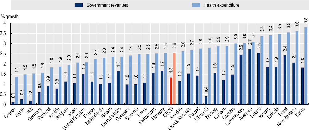
• Projections show that over the next two decades, OECD countries are likely to face a dual challenge of upward pressures on health spending, and constraints on the revenues governments can expect to raise. Growth in health spending from public sources is projected to be twice the average growth in government revenues (2.6% and 1.3% respectively), on average across OECD countries between 2019‑40. Consequently, health spending from public sources is projected to reach 20.6% of government revenues across OECD countries by 2040, an increase of 4.7 percentage points from 2018.

• Health spending from public sources is projected to reach 8.6% of GDP, an increase of 1.8 percentage points from 2018.

• Pressures on health spending are expected to be particularly substantial in Korea and Türkiye (+4% annual growth on average between 2019‑40). On the revenue side, almost no increase in government revenues is projected for Greece, Italy and Japan between 2019‑40.

• Changes in the age structure of the population are likely to have a smaller impact on determining health expenditure as compared to other supply-side factors, notably technological changes and rising incomes. Over the next 20 years, population ageing is expected to increase health spending by 0.2% per year, and to reduce government revenues by 0.2% per year, on average across OECD countries. Changes in the population age structure are projected to decrease government revenues in all OECD countries except New Zealand by 2040.

• Policies that support prevention and promote healthy lifestyles as well as policies that enhance efficiency may rein in projected growth in health spending. Policies to secure the future fiscal sustainability of health systems should also make government revenues more robust to an ageing demographic profile.

3.1. Introduction

Even before COVID‑19, many OECD countries expected that the financing of their health systems would be put under severe pressure over the decades to come. The pandemic has made this outlook even more challenging. Health systems need to be more resilient, so that any future health shocks do not endanger the accessibility and quality of health services. This includes not only being responsive to several “mega-trends” emerging in OECD economies that will affect healthcare – such as population ageing, technological developments, changes in labour markets and family structure, and a more integrated global economy – but also potential health shocks in the future, which include repeated pandemics, anti-microbial resistance, the effects of climate change, disruptions to digital infrastructure, and others that cannot be foreseen.

In addition to these considerable challenges, COVID‑19 has made abundantly clear that health system resilience must also be added as a necessary component to wider economic sustainability. In 2020, the pandemic contributed to a reduction of 3.4% in the size of the world economy (in GDP terms), with OECD countries experiencing reductions as large as 10.8% (OECD, 2021[1]). Looking ahead, repeated future health shocks have the potential to affect economic growth through cumulative impacts if they are not contained and mitigated effectively by health systems.

In this chapter, a new method is used to assess the longer-term fiscal sustainability of health systems. By coupling health spending projections with government revenue projections, the effects of population ageing and income growth on both government revenues and health spending can be simultaneously explored. Analyses that give equal attention to health expenditure and government revenues better capture the need for a whole‑of-government set of policies, addressing in particular the consequences of ageing.

The chapter builds on and extends previous work of health spending by the OECD (de la Maisonneuve and Oliveira Martins, 2013[2]). This chapter develops the health expenditure modelling framework and incorporates additional countries into the analysis. It then adds accompanying analysis on the revenue side, drawing on the revenue buoyancy methodology of (Lagravinese, Liberati and Sacchi, 2020[3]), extending that approach and integrating policy-based revenue scenarios alongside health expenditure projections. Note that this revenue projections approach assumes that past changes to tax policies will persist into the future. The result is a comprehensive set of projections of the future fiscal sustainability of health systems of OECD countries.

To obtain an order of magnitude of the long-term fiscal sustainability of health systems, this chapter is organised as follows. First, it projects health spending from public sources through 2040, accounting for major cost drivers under different scenarios. It then projects government revenues to 2040. Finally, the share of health spending in government revenues is projected up to 2040.

3.2. Projecting health spending from public sources

This chapter focuses on future current health spending from public sources, defined as including spending by compulsory health insurance as well as by government schemes.1 Health spending from private sources of out-of-pocket payments and voluntary health insurance is beyond the scope of this chapter. The projection model uses a component-based approach, which allows projections of five‑year age groups to be disaggregated by the main drivers of spending (Box 3.1). Regression model results provide the value of the coefficients used to project the impact of income, productivity constraints and technological advancements on health spending over time.

Box 3.1. Drivers of health spending

The income effect is measured by the income elasticity of health spending, which captures the percentage change in health expenditure in response to a given percentage change in income. While early studies found income elasticity to be higher than one (health expenditure increasing faster than income), current evidence using international panel data and appropriate regression methods that account for other cost drivers largely find income elasticity of around 0.7‑0.8 for OECD/high-income countries. Evidence generally shows that as countries become richer, income elasticity tends to decrease (Baltagi BH, 2017[4]). Intuitively this means that as countries achieve adequate levels of care and coverage for all, a relatively lower share of income will be allocated to health. However, it is important to note that when GDP is used as a proxy for income, this does not necessarily imply that health expenditure as a share of GDP will decrease, since the income effect does not factor in growth in health spending from other drivers of health spending.

Productivity constraints are measured by the “Baumol variable” (Baumol, 1967[5]), a proxy that captures the impact of lower productivity growth in the health sector relative to other sectors of the economy on health spending. Baumol posited that some sectors of the economy are ‘non-progressive’, meaning they do not benefit from technological advancements as much as other sectors do. Such sectors, including health and education, do not displace labour at the same rate (or at all) when new technologies are implemented, as compared to ‘progressive’ sectors of the economy. In other words, the health sector is labour-intensive and likely to remain so in the coming years. The Baumol effect states that as productivity and wages rise together in ‘progressive’ sectors of the economy, the health sector (being ‘non-progressive’ and thus remaining labour-intensive) will experience wage increases in line with the rest of the economy, but not commensurate productivity increases. In practice, the Baumol variable captures excess (to economy-wide) health price inflation.

Technological progress takes different forms – product, knowledge or process innovation – and represents the most complex driver of healthcare expenditure to model (Chernew and Newhouse, 2012[6]). The challenge technology poses as a driver is twofold: first, endogenous interactions with other drivers of spending are large. Technology affects demographic change, shapes productivity and to some extent reflects consumer demand as incomes rise. Second, such interactions, and indeed technology on its own, are difficult to account for at the macro level: proxies for technology are both scarce and inefficient, particularly for international panels (Marino et al., 2017[7]). In this chapter, the impact of technological progress on health spending is estimated through a time‑specific coefficient, while also acknowledging that some of its effects might be endogenously captured by the income and Baumol effects.

The demographic effect is captured by changes in the population by five‑year age groups over time. Furthermore, as expenditures are concentrated in the last years or months of life independently of the age at which death occurs – commonly referred to as the death-related costs (DRC) hypothesis (Lubitz and Riley, 1993[8]) – costs for non-survivors are assumed to be ten times higher than costs for survivors by five‑year age groups. This expenditure ratio reflects the mid-point of values reported in the literature (Marino et al., 2017[7]). This value of ten is then adjusted over time to reflect country-specific gains in life expectancy. Such dynamic DRCs are used as a proxy to model healthy ageing. The healthy ageing assumption implies that survivors are ageing more healthily (as their health expenditure is lower than non-survivors) and morbidity is compressed towards later age groups (since mortality rates, and therefore expenditure, are higher in older age). Furthermore, death-related costs are adjusted over time to reflect country-specific gains in life expectancy. Given the importance of proximity to death in driving expenditure, the changing patterns of age at death and the increase in life expectancy, the health expenditure of older people falls relative to younger people over time (Cylus, Figueras and Normand, 2019[9]).

3.2.1. Specifications of the health spending projection model

The impact of income, productivity constraints and time‑specific effects on healthcare expenditure is estimated through panel regressions run on historical data (2000‑18) for 33 OECD countries. The base specification uses demography, GDP per capita,2 productivity and a time factor to estimate health expenditure. The dependent variable is current health expenditure per capita from public sources, in real terms and in national currency. Additional controls for demography and technology, as measured by the share of people aged 65 or more in the total population and research and development (R&D) expenditure in the general economy respectively, are also included in the analyses. A dummy variable to account for negative real GDP growth is also used. The regression model uses log-differenced data for all variables, and the preferred specification uses random effects.

The income effect is measured by the income elasticity of health spending, which captures the percentage change in health expenditure in response to a given percentage change in income.3 In the preferred specification, the estimate for the income elasticity of health spending from public sources is 0.767. For projections, this means a 1% increase in potential GDP brings about an average 0.767% increase in health spending, all else being equal. It is important to note this does not necessarily imply that health expenditure as a share of GDP will decrease, since the income effect does not factor in growth in health spending resulting from all other drivers.

Potential productivity constraints are measured by the “Baumol variable”, a proxy that captures the impact of lower productivity growth in the health sector relative to other sectors of the economy on health spending. Historical, country-specific, average growth in wages in the overall economy in excess of productivity per worker in the overall economy was used as the projection proxy of the Baumol effect, and multiplied by the coefficient estimated in the panel regression for the Baumol variable (0.482). This implies a 1% increase in wage growth in excess of productivity growth is translated into a 0.482% increase in health spending from public sources, all else equal. The Baumol variable is capped at 0.01 to 2040. This means that the value of the Baumol variable would decrease linearly to 0.01 from 2018 to 2040 if the mean observed value from 2000 to 2018 for a country is higher than 0.01. If the average growth in wages in excess of productivity per worker is negative, then the Baumol variable equals the annual average productivity growth. This is the case for Greece, Italy, Japan, Portugal and Spain.

Lastly, two proxies for technological progress were used in the regression model. First, expenditure growth on R&D is included. This proxy variable was not significant in regressions for health spending from public sources – in line with the literature – but it did significantly affect other drivers in some of the specifications. Second, year dummies are included. These capture systematic growth that is not taken into account from all other parameters within the model, reflecting in part technological progress. The resulting variable is a year-specific growth for all years in the panel, which are subsequently averaged using a linear weighting that gives more weight to years closer to the base year of the projection and less weight to years further away. The coefficient for this time‑specific effect is 0.004, implying a 0.4% increase in health spending for each year, all else equal. The impact of technological progress on health spending is therefore estimated through the time‑specific coefficient, while also acknowledging that some of its effect might be endogenously captured by the coefficients for income and productivity.

The general equation is as follows:4

$\mathrm{\Delta }\ln {HCE}_{c,t}=\mathrm{ }\alpha +{Demo}_{c,t}+{\beta }_2\mathrm{\Delta }\ln {GDP}_{c,t}+{\beta }_3\left(\mathrm{\Delta }\ln W_{c,t}-\mathrm{\Delta }\ln Y_{c,t}\right)+{\eta }_c+{\tau }_t+{\epsilon }_{c,t}$

The dependent variable HCE is healthcare expenditure per capita in country c for year t; Demo refers to the demographic component; ${\beta }_2$ is the income elasticity of GDP; ${\beta }_3$ is the coefficient of the Baumol variable, measured as wages in the overall economy W in excess of productivity per worker Y; ${\eta }_c$ and ${\tau }_t$ are country and time effects; ${\epsilon }_{c,t}$ is the residual component of the regression.

3.2.2. Projections and scenario analysis

Projections can make an important contribution to better long-term planning. They combine information on well-understood determinants of healthcare spending such as demographic changes, with the impact of broader economic, technological, and social changes. Projections are not forecasts – they do not attempt to estimate what will happen in the future but explore what could happen if existing trends continue or certain events occur. Information on relatively predictable factors, such as the ageing of the population, is often combined with information on more uncertain factors to create scenarios. Scenarios5 describe a range of possible future states of the world by combining different assumptions, for example around policy choices or cost drivers (e.g. new technologies).

In this chapter, a “base” policy scenario projects health spending under the assumption that policies remain similar to how they were before the COVID‑19 pandemic, except for a linear increase of up to 10% in 2040 in the productivity in the health sector as compared to the general economy, which reflects historical trends. The base scenario also models healthy ageing through a reduction in expenditure, on average, for survivors. In the base scenario, a partial dynamic equilibrium is adopted, whereby only half of the gains in life expectancy translate into a reduction of future spending across all age groups.6

Three additional policy scenarios are analysed: “cost control”, “cost pressure” and “healthy ageing”. A “cost control” scenario estimates the extent to which effective cost containment policies can offset health spending drivers. In particular, it assumes a linear increase up to 20% in 2040 in productivity in the health sector (compared to 10% in the base scenario), and a linear decrease up to 10% in 2040 in the income elasticity of health spending (compared to no change in the base scenario) – reflecting that as countries become richer, health systems become more efficient and health outcomes improve. Harnessing new technologies through a better use of Health Technology Assessment, task-shifting and increased generics uptake are some policy examples that best reflect this scenario. A “cost pressure” scenario assumes a linear increase up to 10% in 2040 in income elasticity and constant productivity. Here, ineffective cost containment policies, combined with rising expectations on healthcare, lead to the introduction of expensive new technologies, with insufficient consideration of their cost-effectiveness. While in this scenario quality of care may increase, such gains will come with considerable cost pressures. Finally, a “healthy ageing” scenario assumes that all life expectancy gains translate into years in good health over time, therefore lowering healthcare expenditure for survivors compared to the base scenario. Here, an assumption of implementation of effective policies that strengthen prevention and promote healthy lifestyles is made.

Table 3.1 shows the value of the coefficient of the drivers of the model by scenario. The values of the base year (2018) coefficients of income elasticity, Baumol effect and time effect were estimated through panel regression analyses run on historical data (2000‑18). Note that this chapter analyses projection scenarios that reflect relatively moderate assumptions about the direction of health policies. Chapter 1 analyses the spending implications of more ambitious transformational policies, both those designed to substantially increase health system resilience, and policies targeting radical cuts to ineffective and wasteful spending on health.

Table 3.1. Value of the coefficients of the driver by scenario

	Income elasticity		Baumol effect
Scenario	2018	2040	2018	2040	Healthy ageing multiplier	Time effect
Base	0.767	0.767	0.482	0.434	0.5	0.004
Cost control		0.691		0.386	0.5	0.004
Cost pressure		0.843		0.482	0.5	0.004
Healthy ageing		0.767		0.434	1	0.004

Note: The coefficients of income elasticity, Baumol effect and time effect were statistically significant at 0.01 level.

3.3. Projecting government revenues

Government revenues can be distinguished between tax and non-tax revenues. Taxes are defined by the OECD as compulsory, unrequited payments to the general government. Taxes are calculated through the multiplication of a tax rate to a tax base (e.g. income, property, consumption, payroll, carbon emission, etc.). Whereas non-tax revenues encompass a large heterogeneity of revenue sources, such as intergovernmental grants, interest receipts, property rents, dividends and profits from state‑owned enterprises, and charges and fees from services provided by governments to specific groups (e.g. toll roads, medical service charges).

Government revenues are projected considering two effects: the long-term buoyancy and the changes in the structure of the population. Buoyancy is a coefficient that captures the sensitivity of government revenues to economic activity or the economic cycle. It can be used to project government revenues based on future trends in economic activities as measured by GDP or the output gap. By multiplying the buoyancy coefficient by the expected growth of the proxy at hand, the projected change in government revenues associated with the change in economic activity is captured. Therefore, when using this projection method, it is implicitly assumed that the relationship between revenues and GDP observed in the past in each country is maintained in the future. This relationship includes tax policy reforms implemented in the past. That is, the model relies on past GDP and government revenue data to project government revenues in real terms. It does not account for emerging policy changes or macroeconomic factors, including recent fluctuations in interest rates and inflation, which can have an impact on specific tax bases (such as property values for property taxes).

Changes in the structure of the population refer to the impact of variations in patterns of labour income, asset income and private consumption over the life cycle as people get older. Those changes capture only the changes in the distribution of the population across age groups – and their income and consumption patterns –, whereas the buoyancy effect captures all changes in GDP, including those related to growth in population size.

3.3.1. Estimating government revenues buoyancy coefficients

The following government revenues model is estimated using ordinary least squares:7

${\Delta ln(R}_{c,i})={{\phi }_c+{\alpha }_c{ln(R}_{c,i-1})+{\beta }_c\mathit{ln}\left({GDP}_{c,i-1}\right)+{\rho }_c\Delta ln(GDP}_{c,i})+D_{c,i}+{ϵ}_{c,i}$ (1).

where R, D, c and a refer to government revenues, dummy for negative real GDP growth, country and time, respectively. $\phi$ is an intercept, $\rho$ is the short-run buoyancy, $\alpha$ is the speed of adjustment and $-\beta /\alpha$ is the long-run buoyancy (the coefficient of interest). Variables are in real terms (deflated by the GDP implicit price deflator).

As changes in tax policies are not controlled for when estimating buoyancies, the easiest way to minimise the extent to which these effects are captured by the buoyancy coefficient and reproduced in the projections is by using total revenues, by and large the distribution with the least dispersion and whose values are closest to unity.

Government total revenue buoyancy coefficients vary from 0.41 (Greece) to 1.32 (Korea), with a median of 1.02. This proximity to one satisfies theoretical expectations and is in line with the results of other studies (Koster G, 2017[10]; Deli et al., 2018[11]; Belinga et al., 2014[12]; Dudine and Jalles, 2017[13]), but contrasts with the results found by (Lagravinese, Liberati and Sacchi, 2020[3]), in which buoyancy coefficients had a tendency to be below one.

3.3.2. Scenarios for buoyancy

As a robustness check, three scenarios for the buoyancy coefficients are used. First, a base scenario assumes that estimated buoyancy coefficients remain constant throughout the projection period. Second, a unitary buoyancy scenario posits that revenue growth is equal to GDP growth. Third, an intermediate scenario postulates that estimated buoyancy coefficients converge to one by 2060 (note that the projection period is through 2040). These three scenarios capture the uncertainty regarding the future value of revenue buoyancy coefficients.8

The rationale behind these three scenarios is that keeping buoyancy coefficients constant over the course of two decades may represent a too strong assumption as countries are expected to pursue the same policy path that they followed throughout the period that was used to estimate the buoyancy coefficients (1990‑2018). As this assumption is unlikely, the goal of the first scenario is to provide an overall estimation of what would happen in case countries repeat the same policies. The second reflects the theoretical expectation that in the long-run tax buoyancies must be one, otherwise the government will outgrow the entire economy or will cease to exist, an extremely unlikely situation. The third scenario assumes that there is some inertia in policy paths and, therefore, buoyancies will gradually converge to their theoretical expectation of one by 2060.

3.3.3. Estimating the impact of changes in the population age structure on government revenues

Population ageing affects government revenues through at least two different mechanisms: by affecting overall economic activity (i.e. expected GDP growth), which is intrinsically linked to government revenues; and by affecting tax bases.

National Transfer Accounts (NTA) data from the UN provide age profiles for economic aggregates from the System of National Accounts. Thus, it is possible to estimate the impact of population ageing on certain taxes or tax bases through the following equation:

${\Delta R}_{c,i}=\mathrm{ }\frac{\sum _a{p}_{c,i,a}{r}_{c,b,a}}{\sum _a{p}_{c,\mathrm{ }b,a}{r}_{c,b,a}}-1$ (2).

Where $\Delta R$ refers to the growth rate for a government revenue item or a proxy for it (e.g. a tax base in the case of taxes), $p$ to the population and $r$ to the respective revenue item or its proxy in per capita terms. The subscripts $c$, $i$, $b$ and $a$ refer to the country, the current year of the projection, the base year of the projection and the age group, respectively. It is worth noting that this equation has $r_{c,b}$ both in the numerator and denominator, which means that it assumes that the age profile remains constant over time, an assumption that seems to be plausible in relatively short periods of time.

It is worth noting that when using the tax base to project the impact of population ageing on tax revenues, it is implicitly assumed that tax rates are constant for different age groups. For instance, for income taxes this means that an increase in the income of a certain group of people will lead to the same increase in tax revenues, regardless of the age group of these people. As OECD countries tend to have progressive tax systems, such an assumption of constant tax rates across age groups will tend to generate smaller estimates of tax revenues when an age group with high earners is growing (e.g. people in their late 40s) and larger estimates of tax revenues when an age group with low earners is growing (e.g. the elderly).9 In a similar vein, for consumption taxes this assumption means that tax rates applied to the basket of products consumed by each age group are the same.

Given data limitations, property tax revenues were considered to be invariant to population ageing.10 Revenues under the heading of “non-tax revenues” and “other taxes” are also considered to be invariant to population ageing. That is because they encompass a large variety of revenue sources and, thus, neither a single variable nor a combination of variables in NTA could be used as a proxy for them.

3.3.4. Age profiles

Figure 3.1 shows the age profile for the three tax bases used in the projections model, that is labour income, private assets income and private consumption.

Labour income11 increases slowly when people are in their mid-teenage years (i.e. from the age of 15 onwards), peaking in their 40s and then decreasing rapidly from their 50s until their 80s. Dispersion across OECD countries is rather small, which shows that this pattern is similar across countries. Therefore, countries in which the expected average age of the population over the next 20 years is within the 40‑54 age group are expected to show an increase in aggregate labour income. “Older” countries, on the other hand, are expected to experience a decrease in aggregate labour income due to an increase in the proportion of people aged 50 years and over.

Private asset income increases slowly when people are in their 20s, peaking in their 60s and decreases rather modestly until their 80s. People aged 85 years and over tend to have more private asset income than those under age 40 years. The dispersion is, though, rather large as there are countries in which people aged 85 years and over are in the age group with the highest private asset income while in other countries less than half of them are in the high earning group. As a result, the impact of population ageing on private asset income depends not only on how young the population is but also on the distribution of private assets across age groups.

Private consumption increases when people are born until their 30s and stays rather flat from there on. The dispersion is not large, which indicates that this pattern of consumption is similar across OECD countries. Projected changes in the size and structure of the population are, thus, the most important elements to estimate the impact of population ageing on private consumption.

Figure 3.1.  Distribution of labour income, private asset income and private consumption by age group across OECD countries

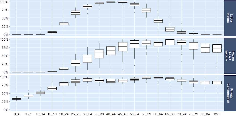
Note: The y axis refers to the value of the respective age group as a percentage of the value of the group with the highest income/consumption while the x axis refers to the age group.

3.3.5. Combining the buoyancy and population age structure effects

To combine the buoyancy and the population age structure effects, the following equation was used:

${TR}_{c,i}=\left(1+\frac{\sum _{a=i}^n{\Delta R}_{c,i}\mathrm{*}{w}_{a,l}}{\sum _{a=1}^n{w}_a}\right)/(1+∆Po{p}_{c,i})\mathrm{*}\left(1+{∆GDP}_{c,i}\mathrm{*}{\theta }_{c,i}\right)-1$ (3)

Where $TR$ refers to total government revenues (real terms), $∆R$ refers to the population ageing effect (as calculated by equation 2), $w$ refers to the portion of total revenues represented by the respective revenue item $a$, $∆GDP$ refers to GDP growth in real terms, $\theta$ refers to the buoyancy for government revenues12 and $∆Pop$ refers to population growth. The subscripts $c$ and $i$ refer to country and time, respectively. ${\theta }_{c,i}$ only changes with time in the third scenario of buoyancy converging to one in 2060.

The separation of the change in the structure of the population from the change in the size of the population avoids double counting the impact of population growth, as this variable is already captured by GDP growth. As a result, the blue equation (in bold) estimated the effect of changes in the structure of the population while the green equation estimated the total buoyancy effect, which includes population growth.

Another key point regards the fact that the projected potential GDP per capita growth rates were adjusted to consider effects from the expected variations in the share of the active population to the total population (for details see (Guillemette and Turner, 2021[14]). Therefore, both the potential GDP per capita used in the estimation of the GDP growth and the modelled relationship between government revenues and GDP are affected by population ageing. As equation 3 captures the effect of these two potential impacts of population ageing on government revenues, the results presented in the next section can be interpreted as an upper bound of the effect of population ageing on government revenues to 2040.

Lastly, it is implicitly assumed that population ageing affects government revenues only through changes in the tax base. In other words, the relationship between tax revenues and tax bases is assumed to be invariant to population ageing. This seems to be a reasonable assumption given that, in theory, this relationship is determined by the tax structure of a country13 and that the main drivers of tax buoyancy are – depending on the type of tax – trade openness, population density, civil liberties, political rights, elements of tax policy, tax rate structure and importance of some industries (Dudine and Jalles, 2017[13]).14

3.3.6. Relevance of government revenue projections in countries where compulsory health insurance is the main financing source of health spending

In this chapter, health spending from public sources as a share of government revenues is used as a proxy to assess the future fiscal sustainability of health systems. In countries like Costa Rica and Germany where social insurance contributions finance a large part of health spending and transfers from government finance a relatively small share of compulsory health insurance spending (Figure 3.2), this proxy may be of less relevance. Further, a few health systems like that of the United States, rely more heavily on private contributions.

Figure 3.2. Financing sources of compulsory health insurance, 2021 (or nearest year)

OECD countries and accession countries with compulsory health insurance contributions representing more than half of total health expenditure

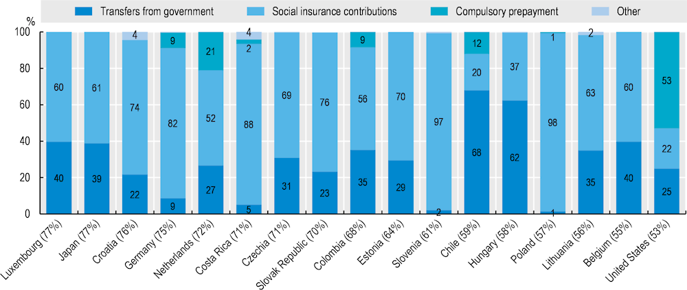
Note: Numbers in brackets indicate the contribution of compulsory health insurance to total health expenditure. Category “Others” includes other domestic revenues and direct foreign transfers.

Source: OECD Health Statistics 2023, https://doi.org/10.1787/health-data-en.

3.4. Results

3.4.1. Projections of health spending from public sources to 2040

Health spending from public sources across the OECD is projected to grow at an average annual rate of 2.6% for 2019‑40 for the base scenario (all results in constant prices, accounting for inflationary effects) 15. This compares with 2.5% for the ‘cost control’, 2.7% for the ‘cost pressure’ and 2.3% for the “healthy ageing” scenarios.

In per capita terms, health spending is projected to grow at an average annual rate of 2.3% for 2019‑40 for the base scenario, 2.2% for the ‘cost control’, 2.4% for the ‘cost pressure’ and 2.1% for the “healthy ageing” scenarios. With an average historical annual growth of 3% for the period 2000‑18, base projections indicate a slowdown in health spending growth compared to the past (Figure 3.3).

Nevertheless, growth in health spending is likely to be significantly higher than GDP per capita growth at 1.2% from 2019‑40. Health spending generally trends GDP growth in terms of its shape, but other spending drivers push it above GDP growth, particularly in the ‘cost pressure’ scenario. This partial relationship between health spending and GDP is consistent with previous OECD analysis of historical spending, which found that cyclical fluctuations in the economy accounted for less than half of the slowdown in health spending during the 2005‑13 period, with the remainder accounted for by policy effects (Lorenzoni et al., 2017[15]).

Given that public health spending is expected to grow faster than GDP, health spending from public sources is projected to reach 8.6% of GDP in 2040 in the base scenario, an increase of 1.8 percentage points compared to 2018, and with a range from 8.5% to 8.8% across the analysed projection scenarios (Table 3.2).

Table 3.2. Health spending from public sources in 2040 under different projection scenarios (OECD average)

Scenario	As percentage of GDP	Percentage point change compared to 2018 value	Average annual growth rate (real terms)	Average annual per capita growth rate (real terms)
Base	8.6%	1.8 percentage points increase	2.6%	2.3%
Cost pressure	8.8%	2 percentage point increase	2.7%	2.4%
Cost control	8.5%	1.7 percentage point increase	2.5%	2.2%
Healthy ageing	8.2%	1.4 percentage point increase	2.3%	2.1%

These results are broadly comparable with other international cross-country analyses. Findings from the Ageing Report (European Commission, 2021[16]), show an increase of 1.3 percentage points of expenditure in 2040 across EU countries in the base scenario (from 8.3% to 9.5%). Comparing the 23 EU members which are also OECD members, our projections show an increase of 1.2 percentage points of health spending as a share of GDP to 2040, whereas the Ageing Report shows an increase of 1.5 percentage points.

Health spending per capita for 2019‑40 is projected to grow above 3.5% per year in Estonia, Korea, Latvia and Lithuania. These are all countries with relatively high GDP growth projections over the period studied. In contrast, the projected growth in Austria and Germany is around 1.5%.

Figure 3.3. Comparison of observed (2000‑18) and projected (base scenario, 2019‑40) average annual percent growth in per capita health spending in real terms by country

Source: OECD Health Statistics, https://doi.org/10.1787/health-data-en, and authors’ compilation.

In the base scenario (Figure 3.4), the demographic effect16 increases health spending by 0.6% per year, on average across the OECD. This amounts to a quarter of the overall projected growth. Note that the demographic effect comprises a “pure age” effect of 0.9% growth. This is moderated by a degree of healthy ageing which decreases spending growth by 0.3% (modelled through dynamic DRCs). Income is the most important driver, accounting for four tenths of annual health spending growth. Productivity constraints (the Baumol effect) account for about one fifth of overall spending growth. Time‑specific effects account for one sixth of health spending growth.

Alternative policy scenarios illustrate the differential impacts spending drivers can have on health spending. For example, productivity constraints increase annual health spending by 0.5% and 0.6% in the ‘cost control and ‘cost pressure’ scenarios respectively, equivalent to around one sixth of overall spending growth. A higher degree of “healthy ageing” means a smaller demographic effect (compared to the other scenarios). The income effect is most dominant in the “healthy ageing” scenario, accounting for 42% of overall spending growth.

Figure 3.4. Annual average percentage growth in health spending in real terms by driver by scenario, OECD, 2019‑40

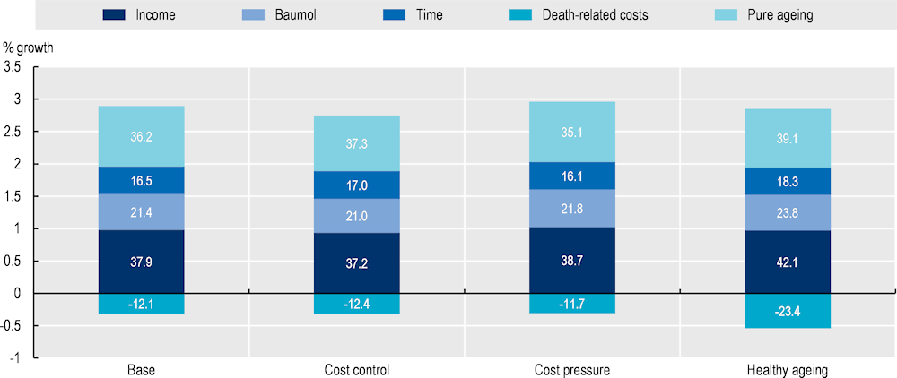
Note: The relative contribution of each driver to growth is reported in percentage within each bar.

Analysing the impact of drivers on spending on a country-by-country basis provides further insights (Figure 3.5). Income effects account for more than 1.5% average annual growth in Estonia, Latvia, Lithuania and Poland, whereas it accounts for less than 0.6% growth in Canada and Italy. Countries with the highest levels of projected GDP growth exhibit the largest income effects in absolute terms, but the relative share of the income effect is naturally dependent on the magnitude of all other effects in any given country.

The Baumol effect, which measures the effect of wages and productivity growth in the economy, is largest and accounts for more than 1% growth in Estonia, Latvia and Lithuania. In contrast, Austria, Greece, the Netherlands and Spain show effects of 0.2% growth or lower. Countries showing a large Baumol effect have experienced wage growth substantially in excess of productivity growth in the general economy – implying that a larger share of health expenditure would need to be allocated to wages in the health sector so as to be on par with wages in the general economy.

Demographic effects are largest in Israel, Korea and Luxembourg – all countries with an absolute growth of 1.5% or more. In contrast, in Latvia and Lithuania demographic change has a negative effect on spending of around 1%. This is largely explained by projected decreases in population numbers in these four countries.

Figure 3.5. Annual average percentage growth in health spending in real terms by driver by country, 2019‑40. Base scenario

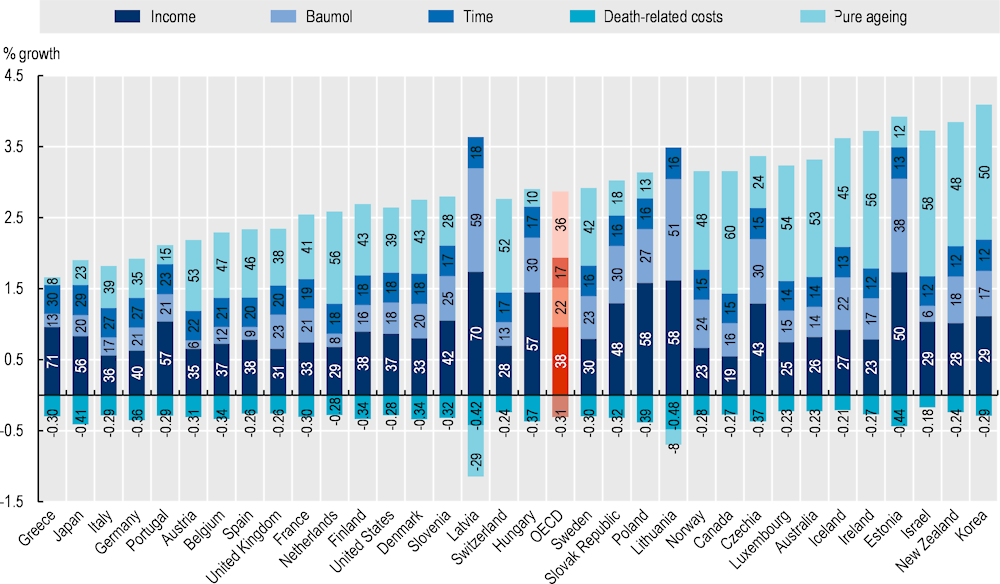
Note: The relative contribution of each driver to growth is reported in percentage within each bar.

3.4.2. Projection of government revenues to 2040

Buoyancy effect on government revenues in 2040

By applying buoyancy coefficients to the potential GDP growth, the cumulative effect of buoyancy on governments’ revenues up to 2040 is estimated.

Figure 3.6 shows the projected government revenues-to-GDP ratios by revenue source in 2040. For all taxes except CIT, the median increase in tax revenues is in line with the increase in GDP growth – the expected change in this ratio varies from a 4% decrease (payroll taxes) to a 1% increase (property taxes), while the CIT revenues-to-GDP ratios are expected to grow by 11%.

It is worth noting that in case these overall trends in tax revenues do occur in the future, they will lead to a change in countries’ tax composition. Revenues from taxes with a higher long-term buoyancy, such as CIT and property taxes, may represent a higher share of total revenues. In contrast, revenues from less buoyant taxes, such as SSCs and GST/VAT, may represent a lower share of total revenues.

Figure 3.6.  Government revenues-to-GDP ratio growth through 2040 due to the buoyancy effect

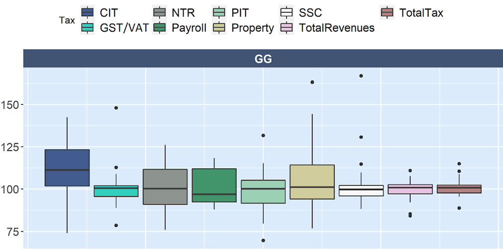
1. PIT, CIT, SSCs, GST/VAT and NTR refer to personal income tax, corporate income tax, social security contributions, good and service tax (or value added tax) and non-tax revenues.

2. On the vertical axis, 100 indicates that the growth in revenues is the same as the growth in GDP.

One important caveat is that projections assume that the relationship between government revenues and GDP between 1990 and 2018 will be the same through 2040. It is unlikely that this relationship will be precisely the same as there were tax reforms in the last decades that are probably not going to be repeated in the future. For instance, CIT revenues were impacted by rate reductions and base broadening over the last decades. Although rates could continue to decrease, the two‑pillar solution to the tax challenges arising from the digitalisation of the economy agreed upon by 137 jurisdictions of the OECD/G20 Inclusive Framework on BEPS in October 2021, will be expected to attenuate the long-term trend of rate reductions, by introducing a multilaterally agreed floor on tax competition with a global minimum effective tax rate of 15%. On the other hand, while opportunities for tax base broadening remain, it is unclear whether the trend towards base broadening witnessed in recent decades will continue. In relation to taxes on goods and services, in the period after the Global Financial Crisis for instance, countries increased their value added tax rates (i.e. a component of taxes on goods and services) to raise more revenues. However, there are decreasing returns to this approach and countries have largely stopped raising their GST/VAT rates (see (OECD, 2020[17]) for an in-depth and recent analysis of tendencies in taxation across OECD countries).

The effect of population ageing on government revenues using NTA

Figure 3.7 breaks down the government revenue projections into two effects: the revenue buoyancy effect (including growth in the size of the population) and the change in the structure of the population. The buoyancy effect is always positive, which was expected given that the GDP growth rate is expected to be positive in all countries in this study. The buoyancy effect varied from 9.5% (Greece) to 82.8% (Australia), with an average of 40.6%.

In contrast, the age structure effect is only positive for New Zealand (a relatively “young” country) and is projected to be negative up to 8% in Slovenia. As a result of changes in the structure of the population, government revenues are expected to decrease – on average – by 4% through 2040.

Figure 3.7. Government revenues cumulative growth rate in real terms due to change in the structure of the population and buoyancy, 2019‑40

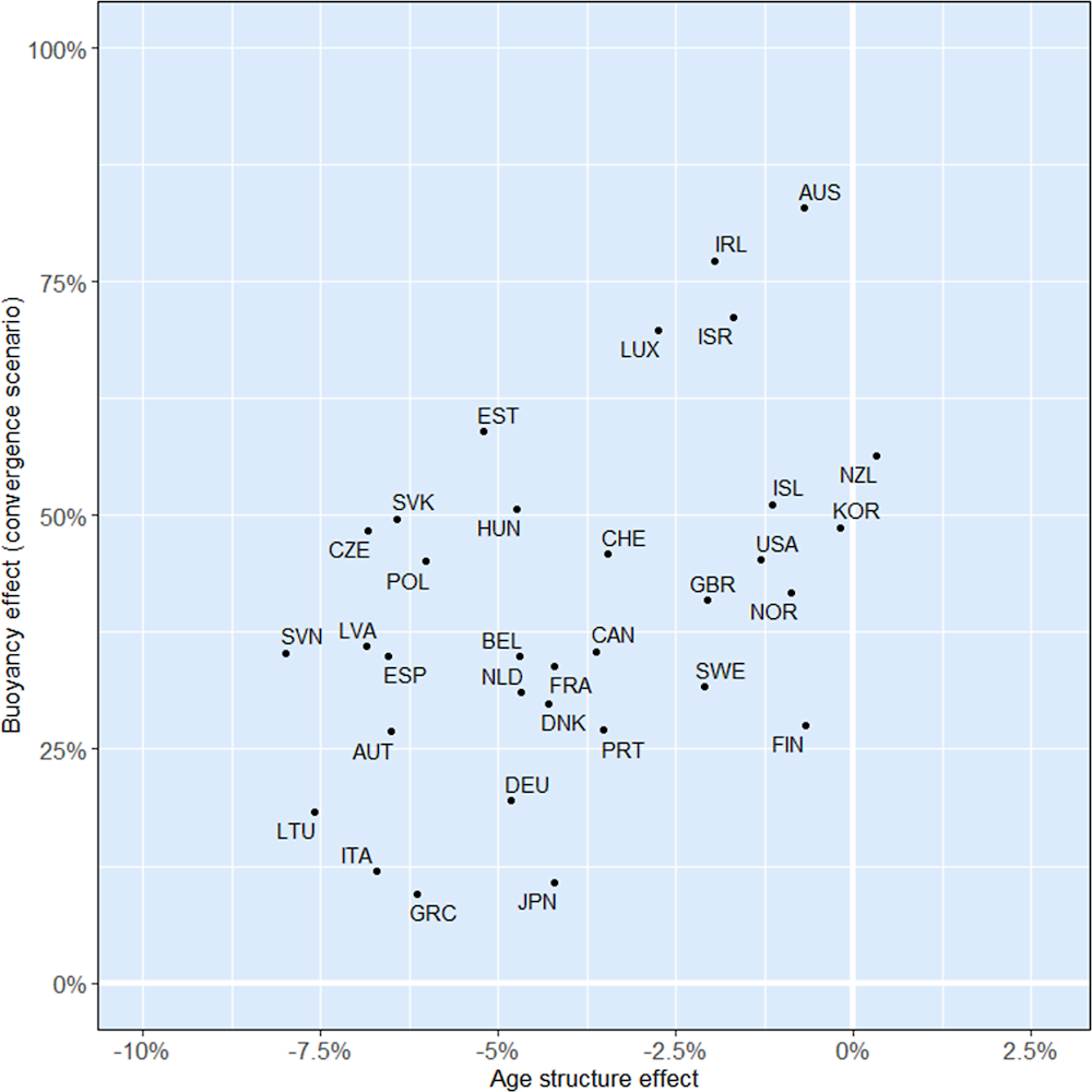
Source: Based on NTA UN, NTA EU. OECD population and GDP projections, OECD Revenue Statistics and SNA.

Figure 3.8 compares growth in government revenues to population growth and potential GDP growth across the three buoyancy scenarios. As many OECD countries are expecting an increase in population, the per capita growth in government revenues was slightly smaller than its growth in levels, in all three scenarios. In the convergence scenario, government revenues are projected to grow – on average – 1.3% per year, while they are expected to slightly decrease as compared to GDP growth (‑0.2% per year).

Figure 3.8. Comparison of government revenues cumulative growth rate across buoyancy scenarios, 2019‑40

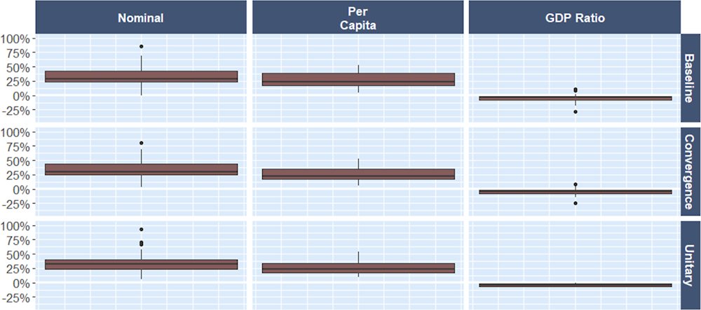
Note: Base scenario refers to the use of the estimated buoyancy throughout the whole projection period; the convergence scenario refers to the scenario in which buoyancy coefficients converge linearly to one in 2060; and the unitary scenario just assumes that buoyancies are unitary.

3.4.3. Fiscal sustainability of health spending

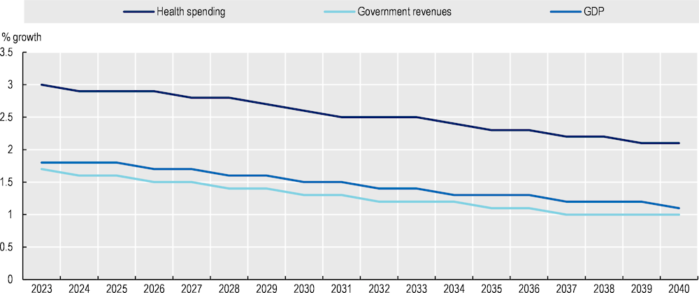
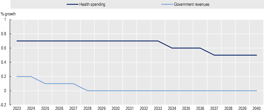
Across the OECD, the mean annual change in health spending in the base scenario is expected to be twice as high as the mean annual change in government revenues from 2023 to 2040 (2.6% versus 1.3%). From 2023 onwards, the growth in health spending is expected to decrease, whereas the decrease in the growth of government revenues is expected to begin in 2025 (Figure 3.9 ). As expected from model specifications, future trends of the growth in health spending and government revenues reflect the projected trend in GDP growth.

Figure 3.9.  Average annual percentage growth in real terms of health spending (base scenario), government revenues (buoyancy convergence scenario) and GDP, OECD, 2023‑40

Health spending is expected to rise at a faster pace than government revenues in all OECD countries. The annual average percentage growth in government revenues is projected to be particularly low in Greece, Italy and Japan at less than 0.3%. In Australia, Ireland and Luxembourg, the annual average percentage growth in government revenues is projected to represent more than three fourths of the annual average growth in health spending (Figure 3.10 ).

Figure 3.10.  Average annual percent growth in real terms of health spending (base scenario) and government revenues (buoyancy convergence scenario) by country, 2023‑40

For all OECD reporting countries, health spending is projected to account for a larger share of total government revenues in 2040 as compared to 2018. On average across the OECD, health spending is projected to represent 20.6% of government revenues in 2040, an increase of 4.7 percentage points from 2018 (Figure 3.11).

Figure 3.11.  Change in the percentage share of health spending (base scenario) in government revenues (buoyancy convergence scenario) by country, 2018 and 2040

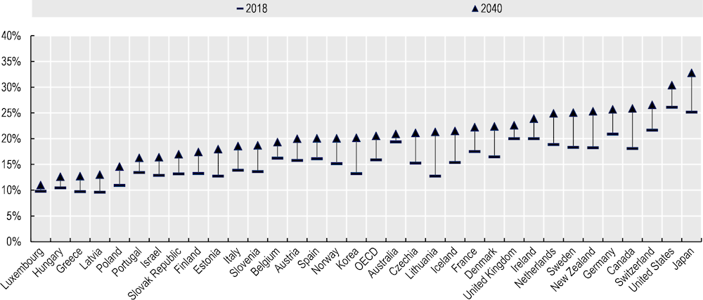
Based on scenario analyses, policies related to enhancing productivity and to improving healthy lifestyles can rein in health spending by 0.3 and 0.8 percentage points of revenues in 2040 respectively.

3.4.4. The impact of changes in the size and structure of the population on health spending and government revenues

Across OECD countries, a decrease in the growth of government revenues due to changes in the size and structure of the population is projected up to 2040. In particular, as from 2028 government revenues – on average – are projected to stabilise. Changes in the size and structure of the population are projected to account for 0.6‑0.7% of health spending growth between 2023 and 2026. Afterwards, the growth in health spending due to the demographic effect is expected to decrease to 0.5%, mainly due to a reduction in the growth rate of the size of the population (Figure 3.12 ).

Figure 3.12.  Average annual percentage growth in real terms of health spending (base scenario) and government revenues (buoyancy convergence scenario) due to change in the size and structure of the population, OECD, 2023‑40

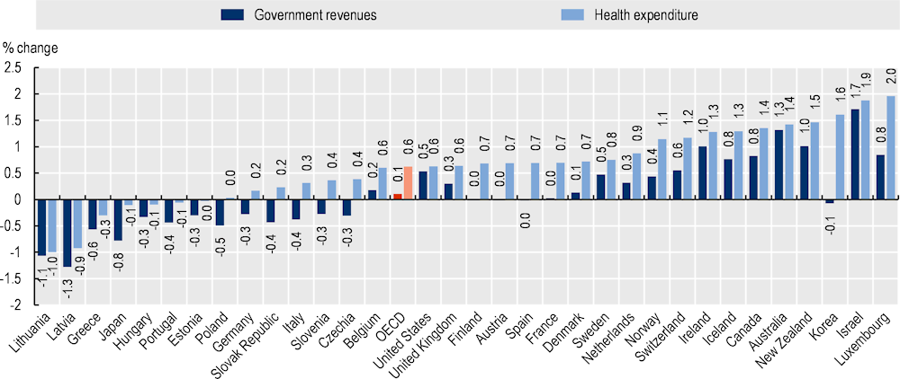
In 15 OECD countries, the change in the size and structure of the population is expected to result in a decrease in government revenues from 2023 to 2040 (Figure 3.13 ). In particular, 13 of those 15 countries are the countries for which a decrease in the size of the population is projected, whereas for the remaining two – Slovenia and Spain – a decrease in the tax base as a result of the change in the structure of the population is projected. In seven of these 15 countries, the highest decrease in the size of the population among the countries in this study is expected to result in a decrease in health spending too.

In two OECD countries – Australia and Israel – the change in the size and structure of the population is projected to result in a growth of government revenues close to the projected growth in health spending. This is due to the highest increase in the population size across OECD countries from 2023 to 2040, and to a share of the population aged 65 years and above lower than OECD average in 2040.

Figure 3.13.  Average annual percentage change in real terms of health spending (base scenario) and government revenues (buoyancy convergence scenario) due to change in the size and structure of the population by country, 2023‑40

3.5. Conclusions

This chapter presents a novel approach to obtain an order of magnitude of the future fiscal sustainability of health systems by coupling health spending from public sources projections with government revenue projections.

As the mean growth in health spending is projected to be twice the mean growth in government revenues (2.6% and 1.3% on average, respectively), health spending from public sources is projected to reach 20.6% of government revenues across OECD countries by 2040, an increase of 4.7 percentage points from 2018.

The findings of this chapter confirm that the role of age per se in determining health expenditure is likely to be small compared to other supply-side factors, such as technological changes and income. The findings of this chapter confirm also that the growth in government revenues slows as populations age. Changes in the size and structure of the population are projected to increase government revenues by 0.1% and health spending by 0.6% per year on average across OECD countries over the next 20 years. This accounts for less than one tenth of the projected growth in government revenues and for one fourth of the growth in health spending respectively. Changes in the structure of the population (i.e. the age‑mix) are projected to decrease government revenues in all OECD countries (except New Zealand) by 2040.

Promoting healthier and more active lifestyles requires action both within and beyond the health sector. Curbing the major risk factors of smoking, alcohol consumption and obesity can reduce associated treatment costs. For example, alcohol prevention policies – such as brief general practitioners’ interventions; taxation; and regulations on opening hours, advertising and drunk-driving – have been shown to reduce costs compared to when associated illnesses are treated when they appear. Similarly, a range of fiscal, regulatory and communication policies have been cost-effective in reducing rates of smoking, obesity and other major risk factors.

Proven policies that can increase productivity include those on health workforce, pharmaceuticals and new technologies. For example, new laws and regulations that extend the scope of practice for non-physicians can produce cost savings with no adverse effects on the quality of care. For pharmaceuticals, price, market entry and prescribing regulations have all helped increase the penetration of generics in the market, thereby saving costs. Health Technology Assessments have the potential to ensure cost-ineffective new technologies are not introduced, and existing cost-ineffective interventions are discontinued. More broadly, stronger price regulation can be effective in reducing health spending.

There is also considerable scope to better harness technological progress, focusing on those technologies that have the potential to increase productivity. Digitalisation can support new care delivery methods that save money, notably in the form of telemedicine and robotic tools for some limited procedures; as well as improving the quality and usefulness of health data.

As a result of GDP growth, government revenues are expected to increase in the long run but, in per capita terms, for most countries this increase will not be as pronounced as it was in the previous decades due to population ageing effects. Policies to make revenues more robust to population ageing may therefore be needed. In particular, reforms to eliminate early retirement pathways and strengthen labour market participation of individuals with a weaker attachment to the labour market could counterbalance future government spending pressures linked to ageing.

The results of projections presented in this chapter are a call to action to change the outcomes predicted by existing trends to secure the future fiscal sustainability of health systems. An important policy message is that addressing fiscal sustainability challenges requires a whole‑of-government set of balanced policies that target both the main driver of health spending and the government revenue generation mechanisms.

References

[4] Baltagi BH, L. (2017), “Health care expenditure and income: a global perspective”, Health Economics, Vol. 26, pp. 863-874, https://doi.org/10.1002/hec.3424.

[5] Baumol, W. (1967), “Macroeconomics of unbalanced growth: the anatomy of urban crisis”, The American Economic Review, Vol. 57/3, pp. 415-426.

[12] Belinga, V. et al. (2014), “Tax Buoyancy in OECD Countries”, IMF Working Papers, Vol. 14/110, p. 1, https://doi.org/10.5089/9781498305075.001.

[6] Chernew, M. and J. Newhouse (2012), Health care spending growth, Elsevier BV, https://doi.org/10.1016/B978-0-444-53592-4.00001-3.

[9] Cylus, J., J. Figueras and C. Normand (2019), Will population ageing spell the end of the welfare state?, European Observatory on Health Systems and Policies, https://eurohealthobservatory.who.int/publications/i/will-population-ageing-spell-the-end-of-the-welfare-state-a-review-of-evidence-and-policy-options-study.

[2] de la Maisonneuve, C. and J. Oliveira Martins (2013), “A Projection Method for Public Health and Long-Term Care Expenditures”, OECD Economics Department Working Papers, No. 1048, OECD Publishing, Paris, https://doi.org/10.1787/5k44v53w5w47-en.

[11] Deli, Y. et al. (2018), Dynamic tax revenue buoyancy estimates for a panel of OECD countries.

[13] Dudine, P. and J. Jalles (2017), “How Buoyant Is the Tax System? New Evidence from a Large Heterogeneous Panel”, Journal of International Development, Vol. 30/6, pp. 961-991, https://doi.org/10.1002/jid.3332.

[16] European Commission (2021), The 2021 Ageing Report, https://doi.org/10.2765/84455.

[14] Guillemette, Y. and D. Turner (2021), “The long game: Fiscal outlooks to 2060 underline need for structural reform”, OECD Economic Policy Papers, No. 29, OECD Publishing, Paris, https://doi.org/10.1787/a112307e-en.

[10] Koster G, P. (2017), Revenue elasticities in euro area countries: an analysis of long-run and short-run dynamics, https://doi.org/10.20955/r.85.67.

[3] Lagravinese, R., P. Liberati and A. Sacchi (2020), “Tax buoyancy in OECD countries: new empirical evidence”, Journal of Macroeconomics, Vol. 63/C, https://doi.org/10.1016/j.jmacro.2020.103189.

[18] Lorenzoni, L. et al. (2023), “Assessing the future fiscal sustainability of health spending in Ireland”, OECD Health Working Papers, No. 161, OECD Publishing, Paris, https://doi.org/10.1787/1f5fadbc-en.

[15] Lorenzoni, L. et al. (2017), “Cyclical vs structural effects on health care expenditure trends in OECD countries”, OECD Health Working Papers, No. 92, OECD Publishing, Paris, https://doi.org/10.1787/be74e5c5-en.

[8] Lubitz, J. and G. Riley (1993), “Trends in Medicare Payments in the Last Year of Life”, New England Journal of Medicine, Vol. 328/15, pp. 1092-1096, https://doi.org/10.1056/nejm199304153281506.

[7] Marino, A. et al. (2017), “Future trends in health care expenditure: A modelling framework for cross-country forecasts”, OECD Health Working Papers, No. 95, OECD Publishing, Paris, https://doi.org/10.1787/247995bb-en.

[1] OECD (2021), OECD Economic Outlook, Interim Report September 2021: Keeping the Recovery on Track, OECD Publishing, Paris, https://doi.org/10.1787/490d4832-en.

[17] OECD (2020), Tax Policy Reforms 2020: OECD and Selected Partner Economies, OECD Publishing, Paris, https://doi.org/10.1787/7af51916-en.

Notes

← 1.  That is, ‘public’ refers to spending by government and schemes of a mandatory nature – i.e. public in this sense indicates the decree of government regulation or control over the uptake of healthcare coverage. Therefore, arrangements in the Netherlands, Switzerland and the United States which are based on an individual obligation to purchase coverage (through private insurers) are included under ‘mandatory’ schemes. It is true that such spending in the case of Switzerland and the United States is not derived from tax revenues or social contributions, and therefore not considered under government spending. However, the discussions about policy options for governments can still apply to an extent given the government ‘control’ over mandates, minimum benefits, etc. while for most countries there is a direct linkage between ‘public’ spending and public sources.

← 2.  For Ireland, the modified GNI is used.

← 3.  Potential GDP is used as a proxy of income in this chapter. The use of this variable allows smoothing large cyclical patterns in GDP. As labour efficiency and trend employment are key components of potential output projections, investments to strengthen health system resilience can support countries reaching their potential output also during shocks. Potential GDP projections are from the OECD Economics Department (Guillemette and Turner, 2021[14]).

← 4.  The first difference of the natural log of all the variables is used to avoid the issue of cointegration.

← 5.  In this chapter, projections are not modelled based on alternative demographic scenarios. For an example of the impact of using alternative demographic scenarios on projecting health spending see (Lorenzoni et al., 2023[18]).

← 6.  The partial dynamic equilibrium coefficient does not have either a mathematical constraint or a largely consistent body of literature behind its estimation. While this means there is no clear recommendation on its plausibility range, it is also the parameter that can be most easily interpreted in terms of scenarios and sensitivity analysis. The parameter can either be estimated or assumed – in the case of 0.5, we assume that half of the gains in life expectancy are translated into DRC growth across all age groups.

← 7.  We allowed coefficients to vary freely across countries because tax policy – which varies significantly across countries – can affect buoyancy, a test for the poolability of observations suggested that we should not pool the revenues of most tax types, including total government revenues, and is consistent with the literature on this topic.

← 8.  We selected 2060 as the convergence year so that this scenario would be compatible with GDP projections from (Guillemette and Turner, 2021[14]).

← 9.  This report also disregards tax policies aimed at some specific age groups, for instance, tax credits targeted to older workers.

← 10.  This means that the age profile for all age groups is the same. This does not mean that ${\Delta R}_{c,i}=0$ as equation 2 will still capture the effect of growth in the size of the population.

← 11.  As it does not include pensions, this might lead to an overestimation of the impact of population ageing on PIT revenues given that in some OECD countries pension income is taxed. In other words, the fact that in our model PIT revenues fully reflect labour income without considering pension income attenuates the drop in PIT revenues when people get older.

← 12.  For Japan, a buoyancy of one was used since the country has a relatively small number of observations (less than 15).

← 13.  It is possible to estimate different tax buoyancies for each age group, but for that purpose, specific tax structure data are needed, which are not available with the required level of detail in a comprehensive and harmonised manner across OECD countries.

← 14.  In addition, to test this assumption further, we regressed the share of population aged 65 years and above onto the buoyancy coefficients in two panel regression settings (with country fixed effects, and country and time fixed effects). In both regressions, the coefficient of the share of population aged 65 years and above was statistically not significant.

← 15.  Results presented in this chapter focus on 33 OECD countries as long-run projections of potential GDP from the OECD Economics Department are not currently available for Chile, Colombia, Costa Rica, Mexico and Türkiye.

← 16.  The demographic effect combines changes in the size and in the structure (i.e. age‑mix) of the population.