Getting to Services in Towns and Villages

2. Services in towns and villages

Abstract

This chapter examines how settlement population and reachability affect service provision. It first shows that the variety and number of services are increasing in settlement size: villages are missing many types of services, while most cities have at least one location (and often more than one) of all services considered. Next, it develops a model to assess the role of reachability in providing different types of services. Smaller settlements (i.e. villages and towns) are partitioned into three categories: close to a city, far from a city but not the largest settlement in the area, and regional centres (far from a city and larger than all other villages and towns nearby). The model results show how service availability varies reachability. Lastly, the chapter compares actual service provision in OECD regions to estimates derived from the model that accounts for regions’ differences in settlement sizes and spatial configurations.

Introduction

Settlements’ reachability may affect their provision of services because residents of each settlement can access services in multiple places. However, such effects likely depend on size asymmetries: a settlement that is larger than surrounding settlements may provide more services than dictated by its own population, while the opposite may occur for smaller settlements that are close to larger ones (Jacobs‐Crisioni, Kompil and Dijkstra, 2023[1]; Cattaneo, Nelson and McMenomy, 2021[2]).

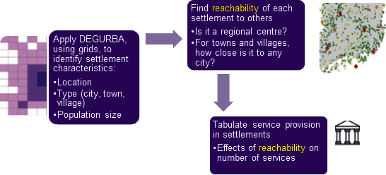
This chapter computes measures of accessibility to other settlements and explores the role that reachability plays in the provision of different types of services (Figure 2.1). To do so, it introduces an empirical model that relates service provision to settlement size, measured as population. The chapter first examines the prevalence of different types of services in smaller settlements like villages and towns compared to cities in 31 OECD countries. Controlling for settlement size, it then investigates reachability measures such as whether a settlement is a regional centre (RC) and whether smaller settlements are close to a city. For example, settlements far from a city that are not RCs may have different levels of service provision from those that are RCs and from similar-sized settlements that are close to a city.

The following section presents modelling results for hospitals, higher education institutions (HEIs), banks, pharmacies and schools to show the impact of the interactions between size and reachability on service provision. Finally, the chapter concludes by comparing actual service provision in regions to that estimated from a model that uses regions’ settlement populations and reachability characteristics as inputs.

Figure 2.1. Analysing the relationship between settlement reachability and service provision

Service provision grows with settlement size (and distance from a city)

Service provision varies for different types of services, settlements and countries. Cities tend to have the highest numbers of services, followed by towns and villages. In absolute numbers, there is a large variation between services. There are noticeable differences between everyday services, those that are common in settlements of all sizes, and less frequently accessed services that are rare in smaller settlements and typically only found in larger places.

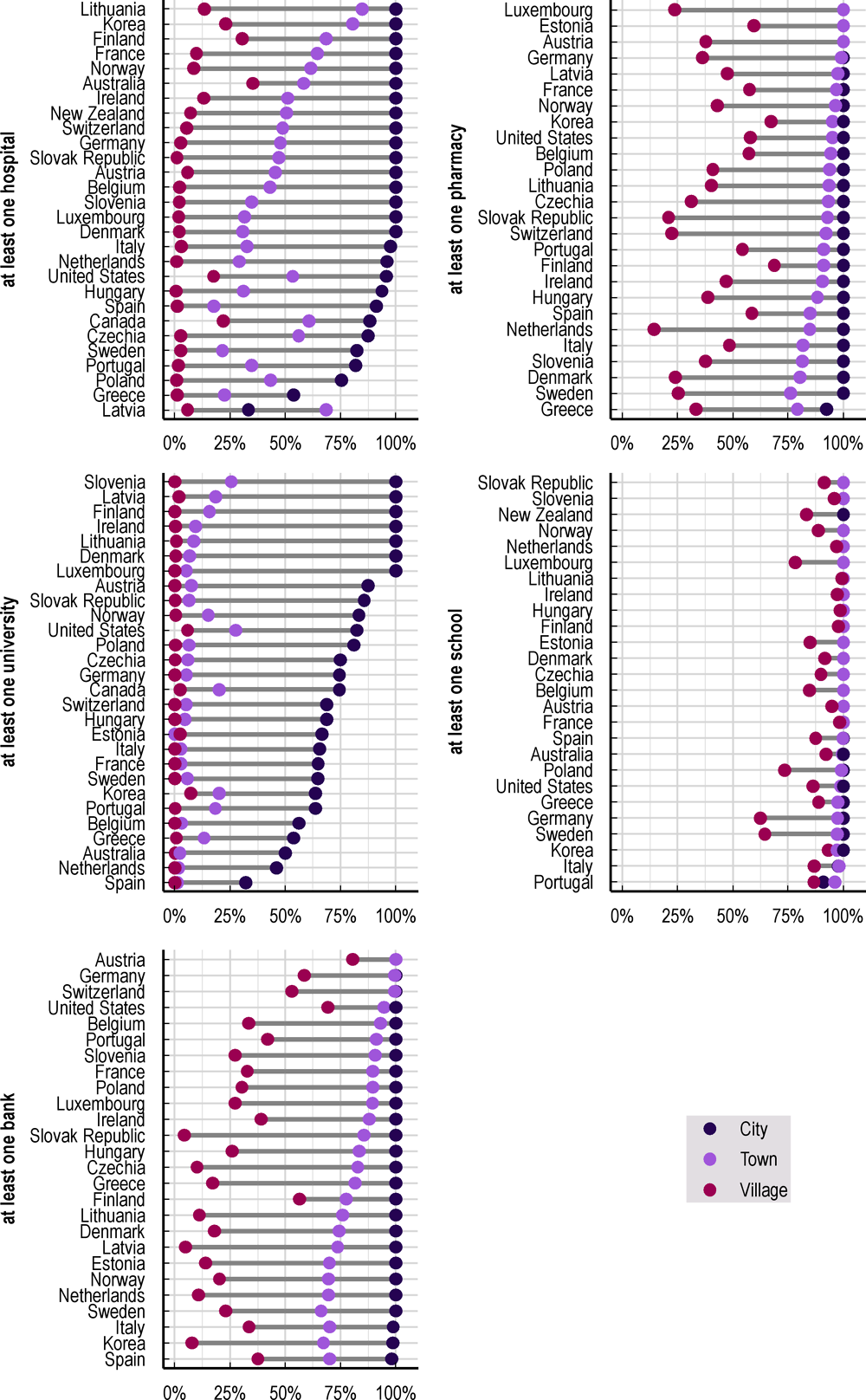
As indicated by Figure 2.2, hospitals and HEIs such as universities are comparatively rare. In contrast, schools, banks and pharmacies – all used on a quasi-daily basis – are relatively common in settlements of all types.

Figure 2.2. Variation in service provision across settlements by type of service

Note: Countries listed in descending order, first by percent of cities with the service and then by percent of towns with the service.

Source: Based on sources in Annex Table 1.A.2 and Annex Table 1.A.3.

Statlink

Almost all settlements have at least one school. In contrast, few villages have a hospital or an HEI close to or within their boundaries. Across OECD countries, HEIs are predominantly found in cities. Thus, hospitals and HEIs tend to have large catchment areas. There are also differences across countries: hospitals are more common in French, Korean or Norwegian towns but rare in Greek, Spanish or Swedish towns.

Larger settlements tend also to have a wider variety of services. Figure 2.3 shows a clear relationship between settlement size and the average number of different services available, tabulated across five main categories (pharmacies, schools, banks, hospitals and HEIs). On average, towns have at least 3 categories of services, while small cities (those with between 50 000 and 250 000 residents) have more than 4 categories. Most larger cities have at least one location in all five service categories, including HEIs. Not only do cities have a greater variety of different service categories, but they also tend to have more locations in each category. In other words, larger settlements have a greater variety and greater number of services. Box 2.1 shows how provision of different types of services, even common ones, differs by degree of urbanisation (DEGURBA).

Figure 2.3. Prevalence of services relative to settlement population

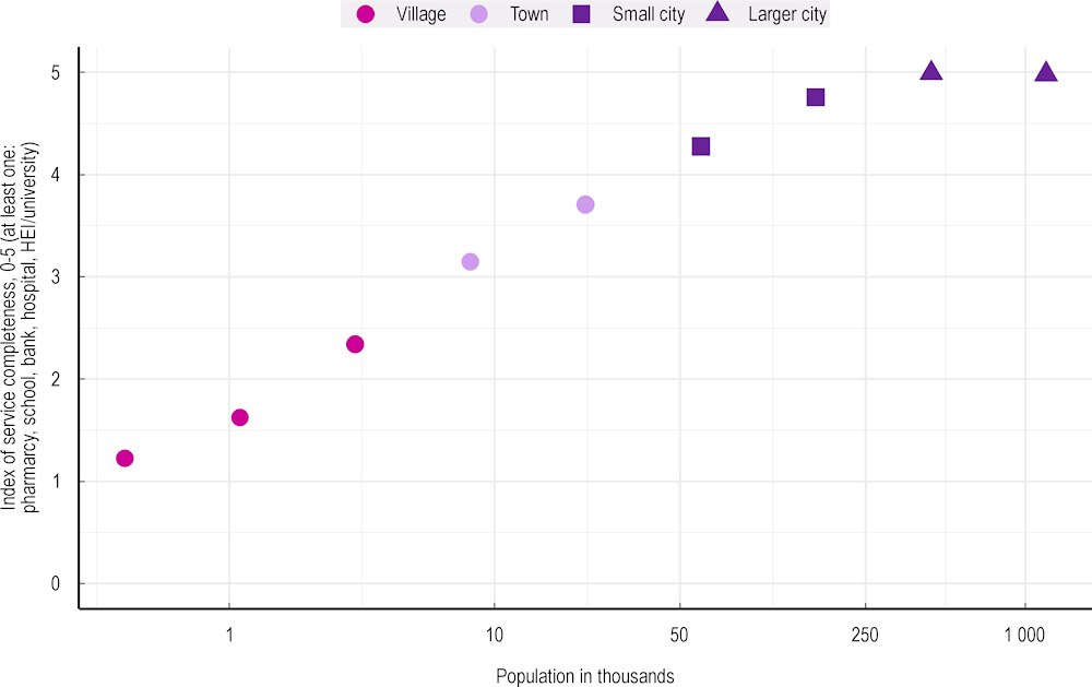
Note: Each marker averages settlements of population defined by population increments over 25 countries with available data.

Source: Based on sources in Annex Table 1.A.2 and Annex Table 1.A.3.

Statlink

A similar pattern emerges when looking at service provision by settlement size in individual countries. Figure 2.4 highlights three countries with large differences by settlement size (Croatia, Slovenia and Slovak Republic) and three with small differences by settlement size (Greece, Italy and Spain). Although villages in Greece, Italy and Spain have a similar number of services as other countries, small cities in these countries lack some services that are available in similar-sized settlements elsewhere. In contrast, most small cities in Croatia, Slovenia and the Slovak Republic have all five services.

Figure 2.4. Prevalence of services relative to settlement population, selected countries

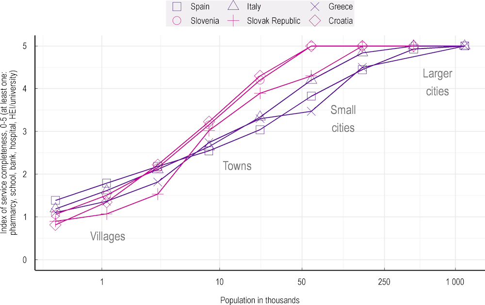
Note: Each marker averages settlements of population defined by population increments.

Source: Based on sources in Annex Table 1.A.2 and Annex Table 1.A.3.

Statlink

Box 2.1. Service provision for essentials and amenities

The case of grocery stores and restaurants in Norway

With their large resident populations, cities typically provide extensive choices among services. Is this the case for both essentials and amenities? An investigation of service locations in Norway reveals two different patterns for grocery stores and restaurants.

Table 2.1 shows municipal-level per capita service provision. There is little difference in grocery stores per capita, whereas restaurants are much more prevalent in cities. Cities have more than twice as many restaurants per capita as rural municipalities and 50% more than intermediate density municipalities.

Table 2.1. Food services in Norway’s municipalities

Average number of service locations per 100 000 residents

DEGURBA Level 1	Grocery stores	Restaurants	Restaurant-to-grocery ratio
Cities/densely populated	50	229	4.58
Intermediate density	52	152	2.92
Rural/thinly populated	55	100	1.82

Source: Based on Statistics Norway (2022[3]), Demographic Data by Municipality.

There are several possible explanations for this pattern. It may be that cities attract residents who value restaurants as an amenity. It may also be that restaurants reach capacity sooner than grocery stores, so each location is individually constrained, whereas grocery stores can serve larger populations within a given geographic proximity. This case study supports the presumption that even relatively common services can have different typical patterns of provision for each service type, as reflected in the regression models utilised throughout this chapter.

Empirical approach to analyse service provision in towns and villages

This chapter analyses spatial differences in service provision across places using the measures of settlement population, reachability and services. It seeks to quantify the relationship between service provision and settlement characteristics like reachability (i.e. being an RC and having access to a city). A regression model in which the provision of services in each settlement is related to its observable characteristics provides insights into these and other spatial patterns (Box 2.2).

Each smaller settlement is categorised as having “Access to a city” if its residents can reach the city within a 30-minute drive. Villages and towns with access to one or more city within 30 minutes cannot be 30‑minute RCs.1 Thus, the reachability of villages and towns can be summarised by three mutually exclusive categories:

1. Access to a city and not an RC – “Access to a city”.

2. No access to a city and not an RC – “No access to a city”.

3. No access to a city and an RC – “Regional centre”.

“Access to a city” acts as the baseline category. These settlements typically have the lowest service counts on average. They are also (by definition) not RCs. The other two categories of small settlements with no access to a city can either be RCs or not, depending on whether there is another nearby town or village that is larger than the settlement itself. Those that are RCs are labelled as “Regional centres” while the rest of towns and villages with no access to a city are classified as “No access to a city”.

Box 2.2. Counting services relative to settlements’ population sizes and reachability

The general regression equation is given as follows:

Equation 2.1. General regression framework

${\mathrm{Y}}_{\mathrm{i},\mathrm{s}}={\mathrm{f}}_{\mathrm{s}}\left[\mathrm{l}\mathrm{n}\left(\mathrm{P}\mathrm{o}{\mathrm{p}}_{\mathrm{i}}\right)\mathrm{ },\mathrm{ }\mathrm{R}\mathrm{e}\mathrm{g}\mathrm{C}\mathrm{e}\mathrm{n}{\mathrm{t}}_{\mathrm{i}\mathrm{ }},\mathrm{A}\mathrm{c}\mathrm{c}\mathrm{e}\mathrm{s}{\mathrm{s}}_{\mathrm{i}}\right]$

The outcome variable $Y$, representing the dependent service location variable, can be a binary indicator or integer. It varies by service type $s$ and settlement $i$. It is modelled via a service-specific regression approach $f_s$. The explanatory variables in $X$ include population size and the two measures of reachability described in Chapter 1 (access to cities and RC status). Regressions are calculated by country.

Schools, banks and pharmacy locations are generally increasing in a settlement’s population. Although some villages have zero counts, other settlements have positive counts of such service locations. The model uses a negative binomial, which is more appropriate when count data has many zeros.

Hospitals and HEIs have relatively few service locations. Many small settlements thus have zero services. An explanation might be small populations and, therefore, missing scale effects. In addition, only large settlements tend to have multiple hospitals or HEIs. Since most settlements have at maximum one hospital or HEI, the regression uses a dummy variable ($Y$=1 if a service is present and 0 if not) to indicate the presence of the service and the estimation uses a logistic regression.

Both regression approaches use the following linear predictor η:

Equation 2.2. Baseline regression

${\mathrm{\eta }}_i=\mathrm{\alpha }+{\mathrm{\beta }}_1\cdot ln\left(Po{p}_i\right)+{\mathrm{\beta }}_2\cdot ln{\left(Po{p}_i\right)}^2+{{\mathrm{\beta }}_3\cdot Acces{s}_i+\mathrm{\beta }}_4\cdot RegCen{t}_i+{\mathrm{\beta }}_5\cdot RegCen{t}_i\cdot ln\left(Po{p}_i\right)+$

${\mathrm{\beta }}_6\cdot RegCen{t}_i\cdot ln{\left(Po{p}_i\right)}^2+u_i$

where $ln\left(pop\right)$ stands for the natural logarithm of the population size of a given settlement i, $Access$ for the remoteness of the settlement and $RegCent$ for the RC status. The regression includes a quadratic population term to capture a possible non-linear relationship between $ln\left(pop\right)$ and service locations per settlement. Finally, an interaction between population and being an RC captures the possibility that larger RCs may have disproportionately more services.

The use of two different modelling approaches results in two different interpretations. For common services, the model results indicate the expected number of services per settlement, given a fixed set of assumptions concerning settlement size and reachability. For uncommon services, they indicate the probability of having at least one service location in a settlement, conditional on settlement size and reachability.

Illustrative results from the model

The model results compare expectations for settlements across the three reachability categories. Modelling helps to identify the role of reachability by disentangling the role of RC status and access to a city from other factors like settlement size, which can vary systematically by reachability (for example, towns that are RCs tend to be larger than towns that are not). Models are estimated by country and service and Annex 2.A reports the full set of results. Schools at country level are highlighted; cross-country averages are then presented for all five services.

This chapter uses benchmark population sizes based on model results for villages and towns to illustrate the effects of reachability on their service provision. As shown in Table 1.2, villages across the OECD have 1 168 inhabitants on average, while towns have nearly 8 500. The regression estimates thus consider a village with 1 000 inhabitants and a town with 10 000 inhabitants to standardise the units of comparison. Figure 2.5 shows the resulting estimates for schools in towns of 10 000 inhabitants by country and reachability category.

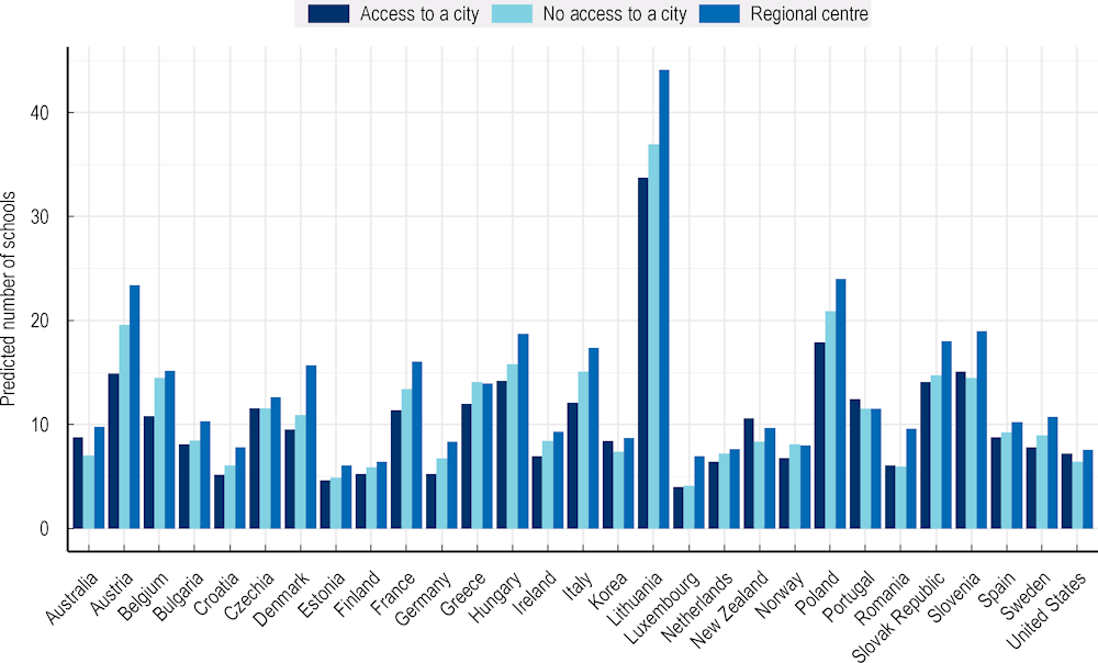
Most countries show a clear reachability gradient for schools, with provision increasing for towns with no access to a city and again for those that are RCs (holding the town size fixed throughout). Two exceptions are Portugal and New Zealand, where the data show slightly fewer school locations in RC towns. Model‑based estimates for common services are often similar to descriptive statistics of service frequency because population is the main driver of service prevalence.

Figure 2.5. Country-level estimates for schools by town reachability

Source: Based on sources in Annex Table 1.A.2 and Annex Table 1.A.3.

Statlink

Figure 2.6. Difference in the expected number of schools relative to towns with access to a city

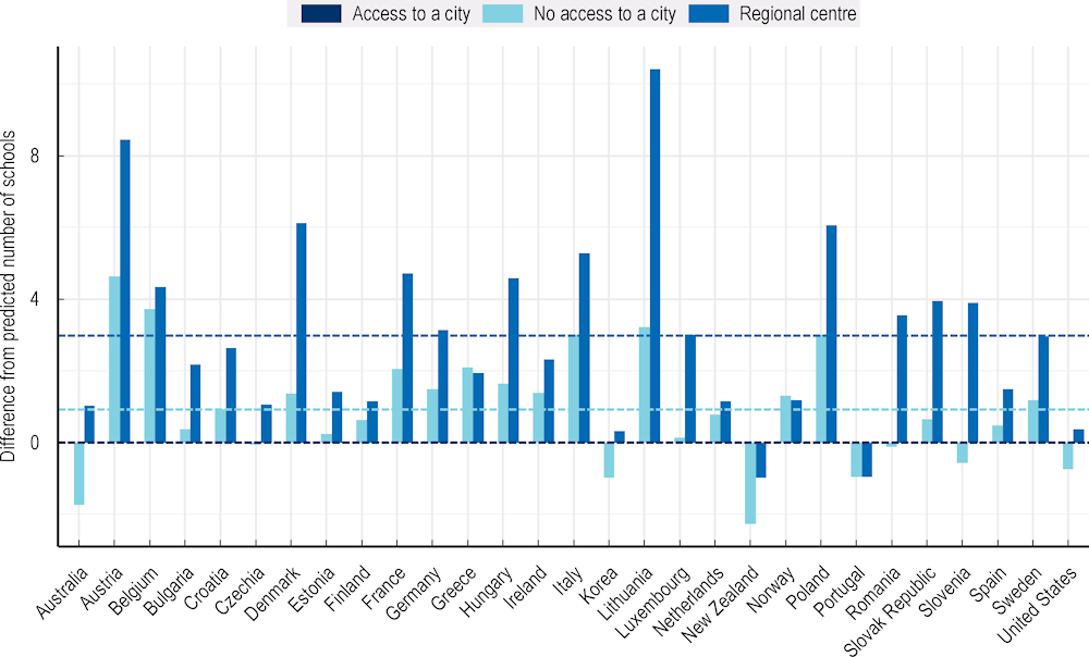
Note: The reference category is towns with “Access to a city”; in other words, towns that are within 30 minutes of a city and thus also not RCs. Dashed lines show the cross-country averages of towns with “No access to a city” and “Regional centre” towns, with colours indicated in the legend. The cross-country average of towns with “Access to a city” is zero, displayed as a horizontal dashed line.

Source: Based on sources in Annex Table 1.A.2 and Annex Table 1.A.3.

Statlink

Figure 2.6 displays the differences in the expected number of schools relative to the baseline category i) a town with “Access to a city” shown in Figure 2.5. The dashed lines indicate the respective cross-country average effects of: ii) having “No access to a city”; and iii) being a “Regional centre”.

In nearly all countries, RCs have more schools compared to non-centres (Figure 2.6). However, in seven countries, towns with access to a city have more schools compared to those without access to a city. Specifically, all of the non-European countries with data on schools (Australia, Korea, New Zealand and the United States) have this pattern, along with Portugal, Romania and Slovenia.

Regional centres have more services than non-centres

The following graphs show the average results of model predictions across all countries. Figure 2.7 summarises three common services: schools, banks and pharmacies. Each panel shows a different service and the x-axis indicates whether the bar depicts a representative town (10 000 inhabitants) or village (1 000 inhabitants). The y-axis is the average change in service locations across OECD countries. Positive values show the number of additional service locations per settlement relative to the baseline town or village close to a city. The average effects for schools in towns correspond to the dashed lines in Figure 2.6. See Annex 2.A for more details.

In general, the patterns in Figure 2.6 show that being an RC is positively correlated with service provision. RC towns have larger numbers of common services compared to the baseline town with access to a city (the baseline category in the graph). Towns that are RCs have, on average, one to two more banks, one more pharmacy and three more schools than similar-sized towns with access to a city. Similarly, RC villages are more likely to have an additional bank, school or pharmacy than non-RC villages.

Smaller settlements that are RCs also have a greater likelihood of uncommon services. Being an RC town doubles the probability of having a hospital from 35% to 78% (Figure 2.8). Being an RC village substantially increases the probability of having a hospital from 3% to 24%. Detailed results show similar patterns across countries (see Annex Table 2.A.4): RCs have higher probabilities for hospitals compared to towns (or villages) that are not RCs. An exception is Korea, where the probability of having a hospital does not vary according to the reachability characteristics of the towns.

Towns and villages far from cities have more services than (similar-sized) settlements close to cities

Service provision in smaller settlements is also positively correlated with having no access to a city. In other words, more remote towns and villages tend to have more services than similar-sized settlements close to a city. For example, using the model to compare towns of similar sizes, those with no access to a city have nearly 1 more school (RC towns have 2.5 more schools) compared to towns with access to a city. Villages with no access to a city also have slightly more of these common services than similar-sized villages with access to a city.

For uncommon services, even those towns that are not RCs – but have no access to a city – are more likely to have a hospital relative to similar-sized towns with access to a city (Figure 2.8). Towns with access to a city have a 35% probability of having a hospital, while that probability rises to 47% for similar-sized non-RC towns without access to a city. For villages, having no access to a city also increases the probability of a hospital relative to villages with access to a city, but being an RC has a much larger impact.

Figure 2.7. Additional services by town (or village) reachability

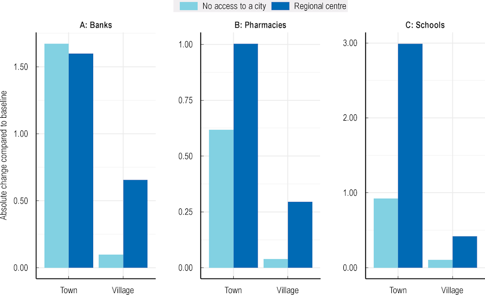
Note: The average town of 10 000 inhabitants with access to a city (baseline category not shown) has 2.8 banks, 3.1 pharmacies and 11 schools. The average village of 1 000 inhabitants with access to a city (category not shown) has 0.3 banks, 0.4 pharmacies and 2 schools.

Source: Simple averages of country-specific estimates in Annex Table 2.A.1 to Annex Table 2.A.3.

Statlink

Figure 2.8. Probability of having a hospital by reachability

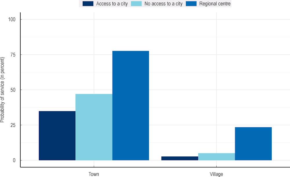
Source: Simple averages of country-specific estimates for towns of 10 000 inhabitants and villages of 1 000 inhabitants (Annex Table 2.A.4).

Statlink

HEIs are scarce (Figure 2.9). The probability of having one is only 5% for towns with access to a city but more than double (12%) for any town without access to a city, regardless of RC status. The effect of reachability on HEI provision is negative for villages: more remote villages and RC villages across the OECD are slightly less likely to have an HEI than villages with access to a city. A case study of Norway (Box 2.3) shows that the presence of one or more HEIs is associated with higher municipality-wide educational attainment.

Figure 2.9. Probability of having an HEI (including university) by reachability

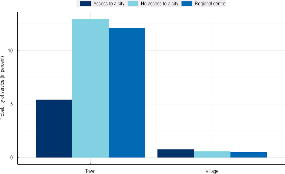
Source: Simple averages of the country-specific estimates for towns of 10 000 inhabitants and villages of 1 000 inhabitants (Annex Table 2.A.5).

Statlink

Box 2.3. Educational outcomes and university access in Norway

Analysing spatial relationships between universities, educational attainment and earnings

Is lower educational attainment a persistent feature of less dense areas or can the presence of a university raise the share of highly educated inhabitants? Norway’s statistical agency, Statistics Norway, has classified all municipalities according to their settlement structure. Moreover, for the purposes of this study, Statistics Norway provided additional information on the prevalence of services such as universities and demographic characteristics of municipal populations including age, marital status, educational attainment, and average earnings in 220 municipalities covering all cities and towns as well as half of the rural areas (Statistics Norway, 2022[3]).1

In Norway’s densely populated municipalities, more than 40% of inhabitants have a tertiary education, whereas a third of the population of semi-dense areas (32%) has a tertiary degree compared to only 25% of the population in primarily rural municipalities (Table 2.2). This contrast is especially pronounced for master’s/doctoral degrees (“long” education as opposed to a bachelor’s level “short” education). In rural municipalities, only 5% of residents have a university degree, compared to 8% in semi-dense municipalities and 15% in cities.

Other characteristics also vary along the rural-urban continuum: The average age of residents in rural and intermediate density municipalities is several years more than in urban municipalities and this difference is statistically significant (using ANOVA analysis). No significant differences were found in the share of married persons. Rural areas have significantly lower average salaries compared to towns and cities; the salary difference increases with DEGURBA (i.e. lowest in villages and highest in cities).

Table 2.2. Summary statistics: Norway’s municipalities

Measure	Rural areas	Towns and semi-dense areas	Cities/densely populated areas
Number of municipalities	145	67	8
Number with at least one university in the municipality	19	30	6
Share of municipalities with at least one university (%)	13	45	75
Population size (mean, thousands)	9	33	202
Average age of residents (years)	43	41	39
Married in population (%)	34	34	33
Tertiary education: short (%)	20	24	28
Tertiary education: long (%)	5	8	15
Average annual earnings (EUR, thousands)	47	50	55

Source: Based on Statistics Norway (2022[3]), Demographic Data by Municipality.

The regression results, described in Annex 2.B, indicate that the presence of a university tends to result in higher educational attainment than predicted from the other territorial characteristics of each municipality (proxied by population and DEGURBA). Higher rates of long tertiary education correspond to higher salaries in semi-dense municipalities but appear to have minimal effects on rural municipalities, while the opposite is true of short education (the effects of short education are positive only for rural municipalities).

Overall, salaries in Norway’s municipalities are increasing with educational attainment, further increasing with municipalities’ population size and the DEGURBA category. However, these patterns are not necessarily causal: higher-educated individuals may be attracted to denser locations that are associated with higher salaries (reverse causality). Greater availability of specialised jobs in dense areas (an omitted variable) may also explain the observed wage-urbanisation gradient.

1. Norway has more than 400 municipalities that differ along the rural-urban continuum. DEGURBA Level 1 offers a classification for small spatial units (local area units, such as municipalities) with at least half of their population in urban centres classified as cities/densely populated areas. At the other extreme, rural/thinly populated areas have more than half of their population in rural grid cells. Towns and semi-dense areas (i.e. intermediate density municipalities) are the remainder.

Source: Statistics Norway (2022[3]), Demographic Data by Municipality.

Variation in service provision across regions

A comparative analysis of service provision by region can be informative for policy makers who are looking to measure regional strengths or shortfalls in services. Estimates from the regression model help extract information about how service provision is expected to relate to settlement sizes and reachability characteristics. Adopting a model-based approach ensures that data on the geography and size of all settlements in a country inform the relationship between settlement size, reachability characteristics and services provision.

Due to data limitations, the model does not account for differences in the size of service locations. Even within countries, the average size of a school, bank or pharmacy could differ by region and settlement type. A key question is whether the average size of services alters the relationship between a settlement’s population and its service provision as measured by the number of locations. Unfortunately, data on the size of individual establishments are often not available, in particular on an international scale. Therefore, the baseline regression model uses only count data without considering service capacity. However, data on the size of individual schools is available for six countries. Box 2.4 uses these cases to explore the effect of size and finds that including size has only a small impact on the regression estimates.

Box 2.4. The role of size in service provision

An example from school sizes in six OECD countries

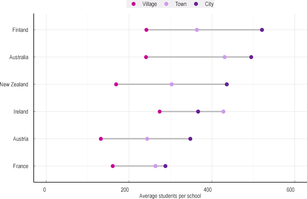
Average service sizes vary across settlements. For example, schools tend to be smallest in villages and increasingly larger in towns and cities, which can imply more service locations per capita in smaller settlements (Figure 2.10). In the six OECD countries with available data, the average number of schools per 100 inhabitants is more than 5 times higher in villages compared to cities.

Figure 2.10. Average school sizes in cities, towns and villages

Comparison of average number of students in schools

Source: Based on school size data obtained from the sources listed in Annex Table 1.A.2.

Statlink

However, this difference in per capita provision does not appear to be due only to differences in school sizes. Instead, some smaller settlements actually have more students than residents. This is not a demographic phenomenon but rather a matter of geography, as many students who go to school in settlements live outside the settlement, especially in sparsely populated areas. The average number of students per inhabitant generally decreases with the settlement population, which means that smaller settlements have a greater need for schools than indicated by their residential populations.

For schools, it was feasible to test whether the omission of size affects the model’s predictions of a number of locations. In six OECD countries, an estimate of average school size (students divided by school locations at the settlement level) was included in the regression model to help predict the number of local schools.

Figure 2.11 shows the predictions for Finland, with and without the size variable.

Figure 2.11. Model estimates with and without school size variables for Finland

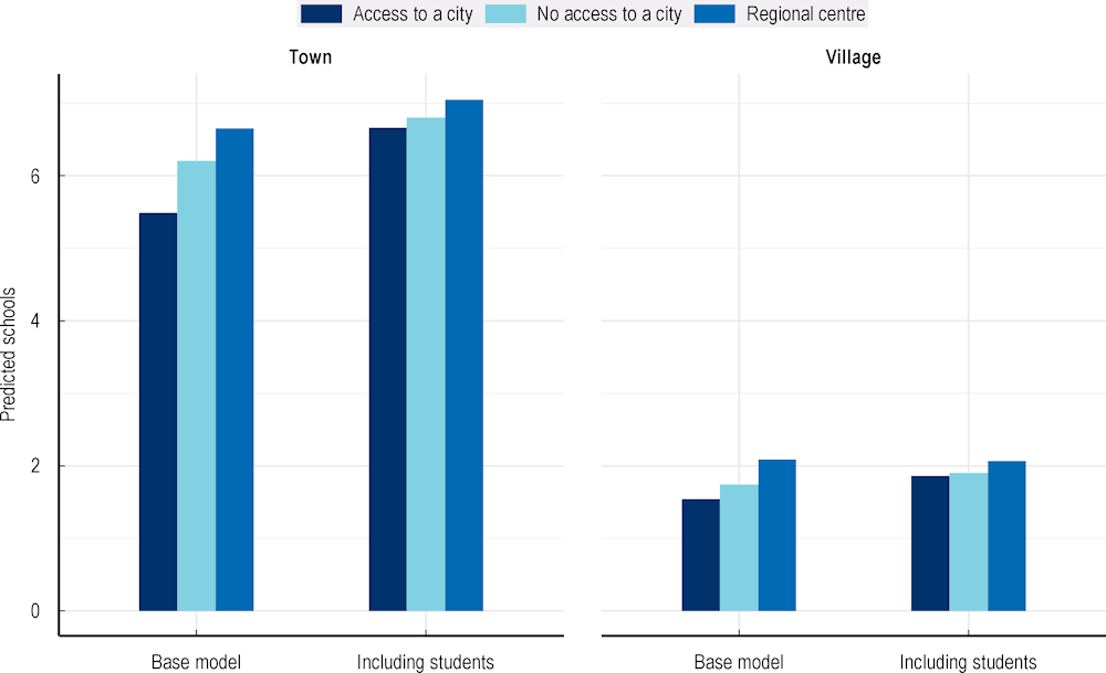
Source: Based on estimates for towns of 10 000 inhabitants and villages of 1 000 inhabitants from the sources listed in Annex Table 1.A.2.

Statlink

Model results indicate that average school size has a small influence on the estimated number of school locations. On average, places with fewer students are predicted to have more schools after accounting for school size. Out of all six countries, Finland has the largest relative change; incorporating school size into the model would increase the number of predicted schools by around 20% in Finish towns and villages with access to cities (approximately 1.2 schools and 0.3 predicted schools more than in the base model respectively). Nevertheless, the conclusions about the effects of reachability are nearly unaffected for Finland and the other five countries with data on number of students.

The regression model can allow for a comparison of expected service prevalence in settlements to actual provision. Positive residuals indicate more services in a given settlement than expected; negative residuals indicate fewer services than expected. Aggregating these residuals to a regional level can inform about the geographic patterns of factors influencing service provision beyond settlement sizes and reachability characteristics.

The maps below show average residuals across TL2 regions, indicating which regions have more or fewer schools and banks in settlements than would be predicted from the geographic configuration of their populations.2 More details and results are in Annex Table 2.C.1. The model estimates for a given region are relative to the rest of the country, so they are informative about within-country but not across-country variation.

There are no apparent trends in the provision of schools in Australia, the European Union and Korea. In the Nordic countries, schools appear to be particularly evenly distributed across TL2 regions, with only a few regions having more or fewer schools than expected, given their settlement networks (Figure 2.12). Conversely, in the United States (Figure 2.13), Florida and Louisiana, along with a handful of western states, have fewer schools than expected, while many midwestern states are close to or above the model’s expectation.

Figure 2.12. Regional variation in actual number of schools: Europe and Korea

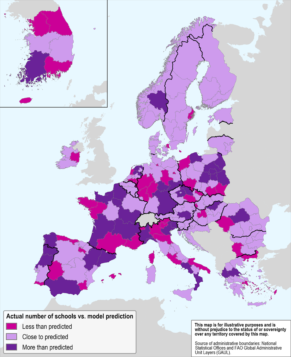
Figure 2.13. Regional variation in actual number of schools: Australia, New Zealand and United States

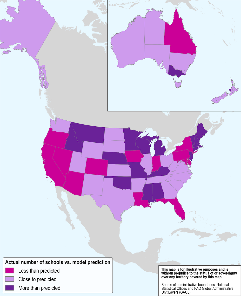
Figure 2.14. Regional variation in actual number of banks: Europe and Korea

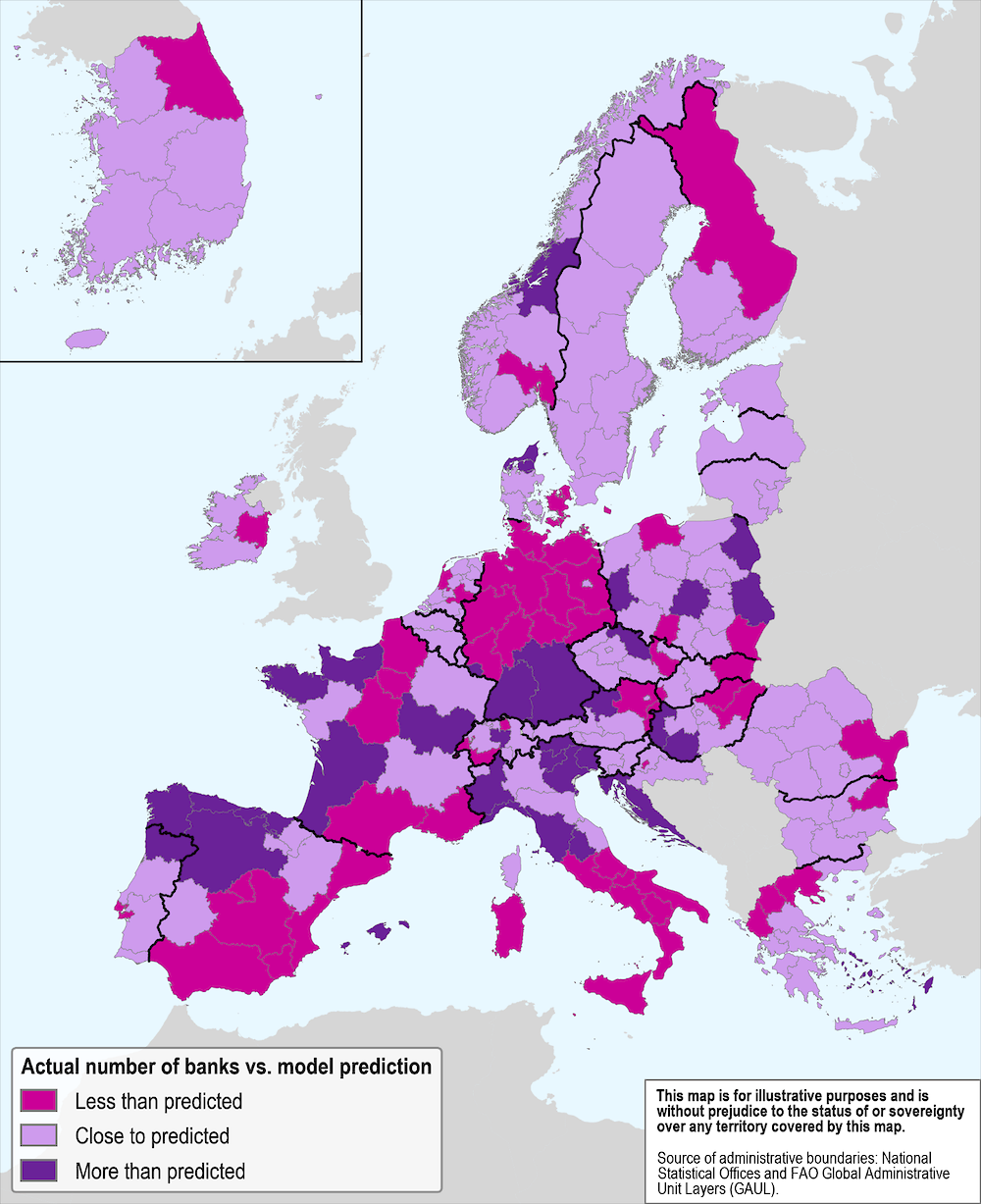
Figure 2.15. Regional variation in actual number of banks: United States

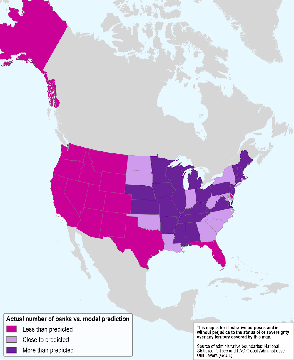
Banks show more geographic clustering than schools. For example, in Figure 2.14, southern regions of Italy and Spain and nearly all northern regions of Germany have fewer banks than expected, while many other areas of those countries have more banks than expected. Similar to banks in the European Union, Figure 2.15 shows the extreme clustering of banks across the United States: all states west of (and including) Texas have fewer banks than expected, while almost all midwestern and eastern states of the country have a number of banks close to or higher than the model estimates. These regional clusters are striking because the model does not account for any features that would make adjacent states similar to each other. Though not shown, patterns of regional clusters also appear for the provision of pharmacies.

The lower spatial correlation of schools may be related to equity considerations because governments are usually more actively involved in the provision of schools, whereas the market plays a comparatively more important role for banks and pharmacies (OECD, 2021[4]). While the regression model in this chapter sheds light on many important aspects of reachability, there are other possible explanations for why certain regions exhibit more or fewer service locations than predicted. For example, modes of transportation can play a role in promoting or limiting actual access (see Chapter 3 for more on transport modes). Settlement networks can also vary in ways beyond those captured by the model.

Conclusions

This chapter shows that the provision of services varies by settlement population, type of service and country. In addition, service provision is found to vary according to settlements’ reachability characteristics. Both measures of reachability – RCs and access to a city – are functionally relevant across all five types of health, financial and education services. The next chapter considers reachability not just from smaller settlements to larger ones but from the area surrounding each settlement. It tabulates the population that can reach any part of a town or village by car and by public transport and looks for a relationship between reachability and the number of services inside the settlement.

Annex 2.A. Additional tables, figures and technical explanations

Annex Table 2.A.1 to Annex Table 2.A.5 below provide country-level detail based on the model estimates. for towns with 10 000 inhabitants and villages with 1 000 inhabitants.

Annex Table 2.A.1. Model prediction of schools by country and settlement size

Model-based estimates from the entire sample of schools in a country’s settlements

Country	Town Access to a city	Town No access to a city	Town Regional centre	Village Access to a city	Village No access to a city	Village Regional centre
Australia	8.77	7.03	9.80	2.76	2.21	1.83
Austria	14.94	19.57	23.38	2.40	3.14	3.10
Belgium	10.79	14.51	15.13	1.11	1.49	1.51
Bulgaria	8.12	8.49	10.30	1.12	1.18	1.73
Croatia	5.16	6.09	7.80	0.71	0.84	0.71
Czechia	11.60	11.55	12.67	1.86	1.85	1.67
Denmark	9.57	10.93	15.68	1.16	1.32	4.18
Estonia	4.64	4.88	6.06	0.92	0.97	1.29
Finland	5.28	5.91	6.42	1.46	1.63	1.90
France	11.38	13.43	16.08	1.74	2.06	2.50
Germany	5.23	6.72	8.37	0.54	0.69	0.74
Greece	12.02	14.11	13.96	2.24	2.63	2.94
Hungary	14.18	15.82	18.77	2.68	2.99	2.66
Ireland	7.00	8.39	9.31	1.49	1.79	2.50
Italy	12.11	15.11	17.39	1.93	2.41	2.66
Korea	8.40	7.43	8.72	4.67	4.12	2.86
Lithuania	33.71	36.93	44.12	5.17	5.66	8.63
Luxembourg	4.01	4.14	7.01	0.68	0.71	1.20
Netherlands	6.46	7.25	7.61	1.08	1.21	1.42
New Zealand	10.64	8.38	9.66	2.07	1.63	1.36
Norway	6.83	8.12	8.01	1.27	1.52	1.63
Poland	17.91	20.91	23.97	1.82	2.12	2.02
Portugal	12.47	11.51	11.50	2.18	2.01	1.58
Romania	6.08	5.96	9.63	0.79	0.78	0.91
Slovak Republic	14.11	14.76	18.05	1.96	2.05	3.27
Slovenia	15.09	14.51	18.98	2.02	1.94	2.14
Spain	8.80	9.28	10.29	1.53	1.61	1.91
Sweden	7.79	8.98	10.75	0.86	0.99	1.43
United States	7.20	6.46	7.57	2.83	2.54	2.89

Note: Values are given as schools per settlement.

Source: Based on sources in Annex Table 1.A.2 and Annex Table 1.A.3.

Annex Table 2.A.2. Model prediction of banks by country and settlement size

Model-based estimates from the entire sample of banks in a country’s settlement

Country	Town Access to a city	Town No access to a city	Town Regional centre	Village Access to a city	Village No access to a city	Village Regional centre
Austria	6.27	8.19	8.84	0.97	1.27	1.66
Belgium	5.09	6.57	6.26	0.42	0.54	1.29
Bulgaria	1.57	2.86	2.21	0.03	0.06	0.23
Croatia	3.64	5.79	6.28	0.13	0.21	1.09
Czechia	2.42	3.46	3.41	0.02	0.03	0.50
Denmark	1.83	3.18	3.68	0.07	0.12	0.93
Estonia	0.71	0.86	2.39	0.10	0.13	0.65
Finland	1.36	2.36	3.07	0.38	0.67	0.99
France	4.51	8.71	7.83	0.26	0.49	1.62
Germany	4.22	5.22	5.90	0.59	0.73	1.15
Greece	2.21	2.94	3.74	0.10	0.13	0.75
Hungary	2.16	2.39	3.65	0.17	0.19	0.50
Ireland	3.03	3.40	4.34	0.41	0.46	1.32
Italy	2.83	2.62	3.73	0.36	0.34	0.63
Korea	1.43	1.33	1.99	0.11	0.11	0.25
Latvia	0.65	4.73	2.43	0.00	0.02	0.37
Lithuania	0.80	2.81	1.97	0.03	0.10	1.32
Luxembourg	5.52	22.97	7.50	0.16	0.66	0.22
Netherlands	0.96	1.07	1.45	0.06	0.07	0.39
Norway	0.96	1.52	2.03	0.08	0.12	0.35
Poland	3.30	3.93	4.93	0.24	0.29	0.65
Portugal	4.84	7.12	7.28	0.38	0.56	1.36
Romania	1.69	1.84	2.64	0.02	0.02	0.18
Slovak Republic	2.99	3.52	4.33	0.00	0.00	0.30
Slovenia	3.27	3.64	5.06	0.19	0.21	1.07
Spain	2.91	3.73	4.10	0.49	0.63	1.29
Sweden	0.92	1.59	2.06	0.11	0.19	1.12
Switzerland	3.75	5.39	7.12	0.48	0.69	2.74
United States	6.45	7.04	8.46	1.61	1.75	2.09

Note: Values are given as banks per settlement.

Source: Based on sources in Annex Table 1.A.2 and Annex Table 1.A.3.

Annex Table 2.A.3. Model prediction of pharmacies by country and settlement size

Model-based estimates from the entire sample of pharmacies in a country’s settlement

Country	Town Access to a city	Town No access to a city	Town Regional centre	Village Access to a city	Village No access to a city	Village Regional centre
Austria	2.69	3.41	2.93	0.22	0.28	0.41
Belgium	3.98	4.74	4.36	0.52	0.62	0.73
Bulgaria	1.30	2.48	1.71	0.06	0.11	0.28
Croatia	3.46	3.07	3.41	0.36	0.32	0.70
Czechia	3.50	4.63	4.45	0.17	0.22	0.49
Denmark	1.18	1.56	1.34	0.10	0.13	0.44
Estonia	4.47	3.23	6.56	0.88	0.63	1.27
Finland	1.43	1.83	2.58	0.43	0.56	0.79
France	3.81	5.44	6.19	0.44	0.63	0.94
Germany	3.50	4.35	5.05	0.20	0.25	0.85
Greece	4.19	4.13	5.37	0.39	0.38	0.97
Hungary	2.46	2.32	3.42	0.30	0.28	0.30
Ireland	4.04	4.98	5.99	0.40	0.50	1.25
Italy	2.53	2.54	3.31	0.44	0.44	0.51
Korea	6.05	6.20	7.93	1.30	1.33	1.03
Latvia	3.30	3.19	4.33	0.57	0.55	0.91
Lithuania	3.88	4.96	4.77	0.44	0.56	0.49
Luxembourg	2.46	8.05	3.25	0.07	0.22	0.09
Netherlands	1.04	1.69	1.03	0.08	0.13	0.03
Norway	2.57	3.48	3.12	0.26	0.35	0.46
Poland	4.41	5.04	5.52	0.40	0.45	0.95
Portugal	3.27	3.90	5.11	0.48	0.58	1.01
Romania	1.39	1.41	2.11	0.08	0.08	0.24
Slovak Republic	3.35	3.83	4.76	0.10	0.11	0.39
Slovenia	2.15	1.66	1.63	0.34	0.26	0.83
Spain	2.90	3.01	3.67	0.58	0.60	0.80
Sweden	1.00	1.63	1.64	0.10	0.16	0.39
Switzerland	2.27	3.75	5.30	0.11	0.17	0.69
United States	4.47	4.48	5.28	1.02	1.02	1.16

Note: Values are given as pharmacies per settlement.

Source: Based on sources in Annex Table 1.A.2 and Annex Table 1.A.3.

Annex Table 2.A.4. Probability of having a hospital by country and settlement

Model-based estimates from the entire sample of hospitals in a country’s settlements

Country	Town Access to a city	Town No access to a city	Town Regional centre	Village Access to a city	Village No access to a city	Village Regional centre
Australia	26.70	58.30	91.76	8.91	27.30	68.88
Austria	38.55	46.14	81.99	2.99	4.03	28.63
Belgium	40.24	59.32	100.00	0.79	1.69	100.00
Bulgaria	65.10	79.70	99.37	0.91	1.91	7.74
Canada	31.30	59.04	92.30	4.74	13.61	45.59
Croatia	20.07	17.57	65.04	2.64	2.25	0.38
Czechia	53.92	68.33	83.26	0.85	1.56	2.82
Denmark	15.76	25.49	75.49	0.55	1.00	57.65
Finland	38.85	63.12	89.63	11.74	26.38	51.92
France	61.11	82.48	94.78	2.75	7.81	37.51
Germany	42.32	58.34	93.58	0.53	1.00	14.04
Greece	5.91	16.62	25.07	0.33	1.03	1.82
Hungary	25.89	26.22	61.98	0.02	0.02	0.04
Ireland	36.10	66.23	91.80	1.78	5.93	71.15
Italy	24.70	32.33	68.64	1.07	1.55	4.87
Korea	80.86	78.79	80.27	20.07	18.09	8.40
Latvia	39.00	68.87	92.93	0.45	1.54	2.25
Lithuania	72.14	78.31	97.77	5.36	7.32	5.01
Luxembourg	27.18	0.00	100.00	2.83	0.00	100.00
Netherlands	20.06	29.34	100.00	0.07	0.11	0.00
New Zealand	41.33	36.37	75.92	1.81	1.47	1.60
Norway	51.42	64.39	81.63	3.47	5.78	3.92
Poland	26.40	47.39	62.46	0.07	0.16	2.48
Portugal	16.76	33.79	75.49	0.08	0.19	4.03
Romania	21.85	22.57	33.70	0.18	0.19	5.87
Slovak Republic	25.00	42.96	90.84	0.13	0.30	0.06
Slovenia	32.32	39.23	47.41	1.58	2.13	0.00
Spain	8.86	10.26	36.15	0.72	0.84	0.26
Sweden	13.87	20.12	41.63	0.00	0.01	36.20
Switzerland	42.60	67.21	92.37	1.84	4.93	8.80
United States	36.86	60.61	85.37	6.57	15.63	56.84

Note: Values are given in percent.

Source: Based on sources in Annex Table 1.A.2 and Annex Table 1.A.3.

Annex Table 2.A.5. Probability of having an HEI by country and settlement size

Model-based estimates from the entire sample of HEIs in a country’s settlements

Country	Town Access to a city	Town No access to a city	Town Regional centre	Village Access to a city	Village No access to a city	Village Regional centre
Australia	2.10	2.22	0.91	0.37	0.39	0.02
Austria	1.88	5.14	7.78	0.08	0.22	0.00
Belgium	1.10	11.63	3.99	0.00	0.05	0.00
Bulgaria	1.44	0.21	2.38	0.81	0.12	0.03
Canada	11.02	11.84	27.38	1.35	1.46	2.75
Croatia	11.46	53.21	32.44	0.00	0.00	0.54
Czechia	4.00	2.16	1.75	0.11	0.06	0.00
Denmark	4.83	3.12	0.00	0.27	0.17	0.00
Estonia	0.00	0.00	0.00	0.00	5.26	0.00
Finland	7.50	52.59	4.38	0.00	0.00	0.00
France	1.84	0.77	1.52	0.16	0.07	0.38
Germany	2.53	3.72	4.91	0.04	0.05	0.08
Greece	9.35	0.57	8.12	2.48	0.14	0.07
Hungary	2.36	2.04	0.55	0.00	0.00	0.00
Ireland	2.78	4.72	6.03	0.25	0.42	0.00
Italy	0.78	1.62	1.99	0.06	0.13	0.01
Korea	20.87	5.47	6.18	9.16	2.16	1.49
Latvia	15.35	0.00	29.36	3.86	0.00	0.00
Lithuania	0.00	9.78	1.07	0.00	0.47	0.00
Luxembourg	0.00	100.00	100.00	0.00	0.00	0.00
Netherlands	0.29	0.00	0.00	0.00	0.00	0.00
Norway	9.80	38.46	14.97	0.00	0.00	2.30
Poland	3.33	3.53	0.87	0.31	0.33	0.00
Portugal	13.74	11.33	18.10	0.05	0.04	0.00
Romania	0.76	0.59	0.45	0.06	0.04	0.01
Slovak Republic	2.67	4.26	0.72	0.07	0.11	0.12
Slovenia	16.15	41.15	42.62	0.00	0.00	4.09
Spain	0.46	0.12	0.03	0.05	0.01	0.00
Sweden	0.90	4.01	3.95	0.00	0.02	0.00
Switzerland	2.13	3.18	9.76	0.06	0.09	0.01
United States	16.27	23.72	43.14	3.94	6.15	3.97

Note: Values are given in percent.

Source: Based on sources in Annex Table 1.A.2 and Annex Table 1.A.3.

Annex Figure 2.A.1 shows the country detail that underlies Figure 2.2. From this detail, it appears villages and towns in Bulgaria and Romania have fewer service categories fulfilled, while those in Finland and the United States have the most. Annex Figure 2.A.1 illustrates how Greece, Italy and Spain differ from Croatia, Slovenia and the Slovak Republic in terms of within-country differences in service provision by settlement size.

Annex Figure 2.A.1. Prevalence of services relative to settlement population, by country

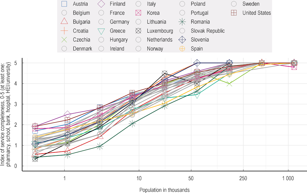
Note: Each marker averages settlements of population defined by population increments.

Source: Based on sources in Annex Table 1.A.2 and Annex Table 1.A.3.

Statlink

Annex 2.B. Educational outcomes in Norway

The following regression examines the variation in educational attainment by Norwegian municipalities relative to each municipality’s population size, DEGURBA and presence of a university. The estimated model between universities and educational attainment is as follows:

Equation 2.3. Education in municipalities

$Y_i={\beta }_0+{{\beta }_1{ln(Pop}_i)\mathrm{ }{+\mathrm{ }\beta }_{2}Rural}_i{\mathrm{ }+\mathrm{ }\beta }_3{Univ}_i+{\epsilon }_i$

where $Yi$ denotes the share inhabitants with tertiary education in municipality $i$ while $Univ$ represents a dummy variable indicating whether the municipality has a university. Since more rural municipalities tend to have lower shares of inhabitants with high educational attainment, a control variable for the degree of urbanisation (whether the municipality is rural) is included. Also, the population size is very different across municipalities. Thus, the logarithm of population is also included as a control. However, city municipalities are omitted from the analysis due to their highly skewed population and relative lack of variation in the data since most municipalities with cities have at least one university.

In Annex Table 2.B.1, the estimated coefficient on population confirms that the share of tertiary educational attainment is lower in municipalities with fewer residents. Moreover, rural municipalities in Norway are associated with even lower shares of higher education, in addition to their smaller populations. While educational attainment is higher in more populated (and more densely populated) areas, a comparison of coefficients in the table above shows a significant correlation between the presence of a university and the overall share of people with higher educational attainment in a municipality. Splitting tertiary education in the regressions into two sub-categories, short and long, reveals that the presence of one or more universities implies a positive coefficient in both cases. However, this result is only significant for short (i.e. bachelor level) educational attainment and not longer (professional or doctoral) degrees. Overall, the presence of a university tends to be associated with higher educational attainment than predicted by the other territorial characteristics of each municipality (proxied by population and degree of urbanisation).

Annex Table 2.B.1. Education model coefficient estimates

Dependent variables:	All tertiary education	Short education	Long education
(Intercept)	14.77**	14.76***	0.02
	-4.74	-2.85	-2.2
log(Population)	1.58**	0.82**	0.76***
	-0.47	-0.28	-0.22
Rural municipality	-4.41***	-2.53***	-1.88***
	-0.93	-0.56	-0.43
University	2.15*	1.55**	0.6
	-0.84	-0.51	-0.39
R2	0.41	0.39	0.37
Adj. R2	0.4	0.38	0.36
Num. obs.	212	212	212

* p < 0.05.

** p < 0.01.

*** p < 0.001.

Source: Based on Statistics Norway (2022[3]), Demographic Data by Municipality.

Follow-up analysis investigates whether the lower rates of tertiary education can help account for why residents of rural municipalities have lower average salaries compared to residents of more urban municipalities. The following model investigates the relationship between income, education and degree of urbanisation (DEGURBA). Average income in each municipality is regressed on the share of inhabitants with higher education and the municipality’s DEGURBA. Furthermore, interaction effects between education and DEGURBA are considered such that education can have a differential impact on salaries depending on territorial characteristics. The logarithm of population acts as a control variable.

Annex Table 2.B.2 shows the relationship between average salary at the municipal level $Y_i$ and municipality characteristics including the share of highly educated inhabitants. As previously, the analysis only considers rural and semi-dense municipalities, not dense urban municipalities.

Salaries are higher in more populated municipalities and also increasing in DEGURBA. The results of this analysis and their interpretation are further described in Box 2.3.

Equation 2.4. Income in municipalities

$Y_i={\beta }_0+{{\beta }_1{ln(Pop}_i)+{\beta }_2{ShortEdu}_i+{\beta }_3{LongEdu}_i+{\beta }_{4}DEGURBA}_i+{\beta }_5{ShortEdu}_i{DEGURBA}_i+{\beta }_6{LongEdu}_i{DEGURBA}_i+{\epsilon }_i$

Annex Table 2.B.2. Earnings model coefficient estimates

	Dependent variable: Average Income
(Intercept)	44 128.63***
	(2 643.13)
	(2 643.13)
log(Population)	390.95**
	(122.18)
Rural municipality (DEGURBA Rural)	-5 134.76*
	(2 555.03)
Tertiary_short_pct	-177.26
	(96.70)
Tertiary_long_pct	654.68***
	(78.29)
DEGURBA Rural: Tertiary_short_pct	311.29**
	(106.08)
DEGURBA Rural:Tertiary_long_pct	-531.16***
	(110.46)
R2	0.50
Adj. R2	0.49
Num. obs.	348

* p < 0.05.

** p < 0.01.

*** p < 0.001.

Source: Based on Statistics Norway (2022[3]), Demographic Data by Municipality.

Annex 2.C. Regional tabulations

Annex Table 2.C.1 provides regional-level tabulations of actual services compared to model estimates, where the latter is based on the size and configuration of the region’s cities, towns and villages.

Results are classified into three categories: More services than predicted; Close to predicted; or Less services than predicted. A TL2 region has more (less) services than predicted if the average Pearson residual of its settlements – representing the difference between actual and predicted services – is statistically different from zero at the 5% level and the average residual is positive (negative). For countries with only one TL2 region (Estonia, Latvia and Luxembourg), service provision is close to predicted by construction because the analysis relies on within-country regressions.

Annex Table 2.C.1. Actual service provision compared to model prediction

Country	Region id	Region name	Banks	Pharmacies	Schools
Australia	AU1	New South Wales	..	..	As predicted
Australia	AU2	Victoria	..	..	More
Australia	AU3	Queensland	..	..	Less
Australia	AU4	South Australia	..	..	As predicted
Australia	AU5	Western Australia	..	..	As predicted
Australia	AU6	Tasmania	..	..	As predicted
Australia	AU7	Northern Territory	..	..	As predicted
Australia	AU8	Australian Capital Territory	..	..	As predicted
Austria	AT11	Burgenland	Less	As predicted	As predicted
Austria	AT12	Lower Austria	Less	As predicted	As predicted
Austria	AT13	Vienna	As predicted	As predicted	As predicted
Austria	AT21	Carinthia	As predicted	More	As predicted
Austria	AT22	Styria	As predicted	More	More
Austria	AT31	Upper Austria	More	Less	As predicted
Austria	AT32	Salzburg	As predicted	As predicted	As predicted
Austria	AT33	Tyrol	As predicted	As predicted	As predicted
Austria	AT34	Vorarlberg	As predicted	As predicted	As predicted
Belgium	BE1	Brussels Capital Region	X	x	x
Belgium	BE2	Flemish Region	As predicted	Less	As predicted
Belgium	BE3	Wallonia	As predicted	More	As predicted
Bulgaria	BG31	North West	As predicted	Less	As predicted
Bulgaria	BG32	North Central	As predicted	As predicted	As predicted
Bulgaria	BG33	North East	Less	As predicted	As predicted
Bulgaria	BG34	South East	As predicted	As predicted	As predicted
Bulgaria	BG41	South West	As predicted	As predicted	Less
Bulgaria	BG42	South Central	As predicted	Less	As predicted
Croatia	HR02	Pannonian Croatia	As predicted	As predicted	As predicted
Croatia	HR03	Adriatic Croatia	More	More	As predicted
Croatia	HR05	City of Zagreb	Less	Less	As predicted
Croatia	HR05	City of Zagreb	Less	Less	As predicted
Croatia	HR06	Northern Croatia	As predicted	As predicted	As predicted
Czechia	CZ01	Prague	As predicted	As predicted	As predicted
Czechia	CZ02	Central Bohemian Region	As predicted	As predicted	More
Czechia	CZ03	Southwest	As predicted	As predicted	As predicted
			Banks	Pharmacies	Schools
Czechia	CZ04	Northwest	As predicted	As predicted	As predicted
Czechia	CZ05	Northeast	More	More	More
Czechia	CZ06	Southeast	As predicted	Less	Less
Czechia	CZ07	Central Moravia	Less	As predicted	As predicted
Czechia	CZ08	Moravia-Silesia	As predicted	As predicted	Less
Denmark	DK01	Capital City Region	Less	As predicted	Less
Denmark	DK02	Zealand	Less	As predicted	As predicted
Denmark	DK03	Southern Denmark	As predicted	More	As predicted
Denmark	DK04	Central Jutland	As predicted	As predicted	As predicted
Denmark	DK05	Northern Jutland	More	As predicted	As predicted
Estonia	EE00	Estonia	As predicted1	As predicted1	As predicted1
Finland	FI19	Western Finland	As predicted	As predicted	As predicted
Finland	FI1B	Helsinki-Uusimaa	As predicted	As predicted	As predicted
Finland	FI1C	Southern Finland	As predicted	As predicted	As predicted
Finland	FI1D	Eastern and Northern Finland	Less	As predicted	As predicted
Finland	FI20	Åland	As predicted	As predicted	As predicted
France	FR1	Île-de-France	Less	Less	More
France	FRB	Centre - Val de Loire	Less	As predicted	As predicted
France	FRC	Bourgogne-Franche-Comté	More	More	More
France	FRD	Normandy	More	As predicted	More
France	FRE	Hauts-de-France	Less	Less	More
France	FRF	Grand Est	As predicted	Less	As predicted
France	FRG	Pays de la Loire	As predicted	Less	Less
France	FRH	Brittany	More	As predicted	Less
France	FRI	Nouvelle-Aquitaine	More	More	More
France	FRJ	Occitanie	Less	As predicted	Less
France	FRK	Auvergne-Rhône-Alpes	As predicted	As predicted	More
France	FRL	Provence-Alpes-Côte d’Azur	Less	Less	Less
France	FRM	Corsica	As predicted	As predicted	Less
Germany	DE1	Baden-Württemberg	More	Less	As predicted
Germany	DE2	Bavaria	More	As predicted	More
Germany	DE3	Berlin	As predicted	Less	Less
Germany	DE4	Brandenburg	Less	More	As predicted
Germany	DE5	Bremen	As predicted	Less	As predicted
Germany	DE6	Hamburg	Less	As predicted	Less
Germany	DE7	Hesse	Less	Less	Less
Germany	DE8	Mecklenburg-Vorpommern	Less	More	As predicted
Germany	DE9	Lower Saxony	Less	As predicted	As predicted
Germany	DEA	North Rhine-Westphalia	Less	Less	Less
Germany	DEB	Rhineland-Palatinate	Less	Less	Less
Germany	DEC	Saarland	More	More	As predicted
Germany	DED	Saxony	Less	More	More
Germany	DEE	Saxony-Anhalt	Less	More	Less
Germany	DEF	Schleswig-Holstein	Less	As predicted	As predicted
Germany	DEG	Thuringia	Less	More	More
Greece	EL30	Attica	As predicted	As predicted	Less
Greece	EL41	North Aegean	As predicted	As predicted	As predicted
Greece	EL42	South Aegean	More	More	Less
Greece	EL43	Crete	As predicted	More	As predicted
Greece	EL51	Eastern Macedonia, Thrace	As predicted	As predicted	Less
Greece	EL52	Central Macedonia	Less	Less	As predicted
Greece	EL53	Western Macedonia	Less	Less	As predicted
			Banks	Pharmacies	Schools
Greece	EL54	Epirus	Less	As predicted	More
Greece	EL61	Thessaly	As predicted	Less	More
Greece	EL62	Ionian Islands	As predicted	As predicted	As predicted
Greece	EL63	Western Greece	As predicted	As predicted	As predicted
Greece	EL64	Central Greece	As predicted	As predicted	As predicted
Greece	EL65	Peloponnese	As predicted	As predicted	As predicted
Hungary	HU11	Budapest	As predicted	As predicted	As predicted
Hungary	HU12	Pest	As predicted	As predicted	As predicted
Hungary	HU21	Central Transdanubia	As predicted	As predicted	Less
Hungary	HU22	Western Transdanubia	More	More	As predicted
Hungary	HU23	Southern Transdanubia	More	More	As predicted
Hungary	HU31	Northern Hungary	Less	Less	More
Hungary	HU32	Northern Great Plain	Less	Less	As predicted
Hungary	HU33	Southern Great Plain	As predicted	As predicted	As predicted
Ireland	IE04	Northern and Western	As predicted	As predicted	As predicted
Ireland	IE05	Southern	As predicted	As predicted	As predicted
Ireland	IE06	Eastern and Midland	Less	As predicted	Less
Italy	ITC1	Piedmont	More	More	More
Italy	ITC2	Aosta Valley	As predicted	More	Less
Italy	ITC3	Liguria	More	More	More
Italy	ITC4	Lombardy	As predicted	Less	Less
Italy	ITF1	Abruzzo	Less	As predicted	As predicted
Italy	ITF2	Molise	Less	As predicted	As predicted
Italy	ITF3	Campania	Less	Less	More
Italy	ITF4	Apulia	Less	Less	Less
Italy	ITF5	Basilicata	Less	Less	As predicted
Italy	ITF6	Calabria	Less	Less	More
Italy	ITG1	Sicily	Less	More	As predicted
Italy	ITG2	Sardinia	Less	Less	As predicted
Italy	ITH1	Province of Bolzano-Bozen	More	More	Less
Italy	ITH2	Province of Trento	More	More	Less
Italy	ITH3	Veneto	More	More	More
Italy	ITH4	Friuli-Venezia Giulia	More	More	More
Italy	ITH5	Emilia-Romagna	As predicted	As predicted	Less
Italy	ITI1	Tuscany	More	More	As predicted
Italy	ITI2	Umbria	More	More	As predicted
Italy	ITI3	Marche	As predicted	Less	As predicted
Italy	ITI4	Lazio	Less	Less	Less
Korea	KR01	Capital Region	As predicted	Less	Less
Korea	KR02	Gyeongnam Region	As predicted	Less	Less
Korea	KR03	Gyeongbuk Region	As predicted	As predicted	As predicted
Korea	KR04	Jeolla Region	As predicted	More	More
Korea	KR05	Chungcheong Region	As predicted	As predicted	As predicted
Korea	KR06	Gangwon Region	Less	As predicted	Less
Korea	KR07	Jeju	As predicted	Less	Less
Latvia	LV00	Latvia	As predicted1	As predicted1	..
Lithuania	LT01	Vilnius Region	As predicted	Less	As predicted
Lithuania	LT02	Central and Western Lithuania	As predicted	As predicted	As predicted
Luxembourg	LU00	Luxembourg	As predicted1	As predicted1	As predicted1
Netherlands	NL11	Groningen	As predicted	As predicted	More
Netherlands	NL12	Friesland	As predicted	Less	More
Netherlands	NL13	Drenthe	As predicted	As predicted	As predicted
			Banks	Pharmacies	Schools
Netherlands	NL21	Overijssel	As predicted	As predicted	More
Netherlands	NL22	Gelderland	Less	As predicted	As predicted
Netherlands	NL23	Flevoland	As predicted	Less	More
Netherlands	NL31	Utrecht	As predicted	As predicted	As predicted
Netherlands	NL32	North Holland	Less	Less	Less
Netherlands	NL33	South Holland	As predicted	As predicted	As predicted
Netherlands	NL34	Zeeland	As predicted	More	As predicted
Netherlands	NL41	North Brabant	As predicted	As predicted	Less
Netherlands	NL42	Limburg	As predicted	As predicted	Less
New Zealand	NZ11	Northland Region	..	..	As predicted
New Zealand	NZ12	Auckland Region	..	..	As predicted
New Zealand	NZ13	Waikato Region	..	..	As predicted
New Zealand	NZ14	Bay of Plenty Region	..	..	As predicted
New Zealand	NZ15	Gisborne Region	..	..	As predicted
New Zealand	NZ16	Hawke's Bay Region	..	..	As predicted
New Zealand	NZ17	Taranaki Region	..	..	More
New Zealand	NZ18	Manawatu-Wanganui Region	..	..	As predicted
New Zealand	NZ19	Wellington Region	..	..	As predicted
New Zealand	NZ21	Tasman-Nelson-Marlborough	..	..	As predicted
New Zealand	NZ22	West Coast Region	..	..	As predicted
New Zealand	NZ23	Canterbury Region	..	..	As predicted
New Zealand	NZ24	Otago Region	..	..	As predicted
New Zealand	NZ25	Southland Region	..	..	As predicted
Norway	NO02	Hedmark and Oppland	As predicted	More	More
Norway	NO06	Trøndelag	More	More	As predicted
Norway	NO07	Northern Norway	As predicted	Less	As predicted
Norway	NO08	Oslo and Viken	Less	As predicted	As predicted
Norway	NO09	Agder and Sør-Østlandet	As predicted	As predicted	As predicted
Norway	NO0A	Western Norway	As predicted	Less	As predicted
Poland	PL21	Lesser Poland	As predicted	As predicted	Less
Poland	PL22	Silesia	As predicted	Less	As predicted
Poland	PL41	Greater Poland	As predicted	As predicted	As predicted
Poland	PL42	West Pomerania	As predicted	As predicted	Less
Poland	PL43	Lubusz	More	As predicted	As predicted
Poland	PL51	Lower Silesia	As predicted	As predicted	Less
Poland	PL52	Opole region	Less	Less	As predicted
Poland	PL61	Kuyavian-Pomerania	As predicted	As predicted	As predicted
Poland	PL62	Warmian-Masuria	As predicted	Less	As predicted
Poland	PL63	Pomerania	Less	Less	More
Poland	PL71	Lodzkie	More	More	More
Poland	PL72	Swietokrzyskie	As predicted	As predicted	As predicted
Poland	PL81	Lublin Province	More	More	More
Poland	PL82	Podkarpacia	Less	As predicted	Less
Poland	PL84	Podlaskie	More	As predicted	More
Poland	PL91	Warsaw's capital city	As predicted	As predicted	More
Poland	PL92	Mazowiecki region	As predicted	As predicted	More
Portugal	PT11	North	More	More	More
Portugal	PT15	Algarve	As predicted	As predicted	Less
Portugal	PT16	Central Portugal	As predicted	As predicted	More
Portugal	PT17	Metropolitan area of Lisbon	Less	As predicted	As predicted
Portugal	PT18	Alentejo	As predicted	Less	As predicted
Portugal	PT20	Autonomous Region of the Azores	As predicted	As predicted	Less
			Banks	Pharmacies	Schools
Portugal	PT30	Autonomous Region of Madeira	As predicted	As predicted	Less
Romania	RO11	North West	As predicted	As predicted	As predicted
Romania	RO12	Center	As predicted	More	More
Romania	RO21	North East	As predicted	Less	As predicted
Romania	RO22	South East	Less	As predicted	As predicted
Romania	RO31	South - Muntenia	As predicted	As predicted	As predicted
Romania	RO32	Bucharest - Ilfov	As predicted	As predicted	As predicted
Romania	RO41	South West Oltenia	As predicted	As predicted	As predicted
Romania	RO42	West	As predicted	As predicted	Less
Slovak Republic	SK01	Bratislava Region	Less	As predicted	Less
Slovak Republic	SK02	West Slovakia	As predicted	More	As predicted
Slovak Republic	SK03	Central Slovakia	As predicted	As predicted	As predicted
Slovak Republic	SK04	East Slovakia	Less	Less	As predicted
Slovenia	SI03	Eastern Slovenia	As predicted	As predicted	As predicted
Slovenia	SI04	Western Slovenia	As predicted	As predicted	As predicted
Spain	ES11	Galicia	More	More	More
Spain	ES12	Asturias	More	As predicted	Less
Spain	ES13	Cantabria	More	As predicted	Less
Spain	ES21	Basque Country	More	More	As predicted
Spain	ES22	Navarra	As predicted	As predicted	As predicted
Spain	ES23	La Rioja	As predicted	Less	Less
Spain	ES24	Aragon	As predicted	Less	More
Spain	ES30	Madrid	Less	Less	As predicted
Spain	ES41	Castile and León	More	As predicted	As predicted
Spain	ES42	Castile-La Mancha	Less	Less	As predicted
Spain	ES43	Extremadura	As predicted	As predicted	Less
Spain	ES51	Catalonia	Less	More	More
Spain	ES52	Valencia	Less	Less	As predicted
Spain	ES53	Balearic Islands	More	As predicted	Less
Spain	ES61	Andalusia	Less	Less	More
Spain	ES62	Murcia	Less	Less	Less
Spain	ES63	Ceuta	As predicted	As predicted	As predicted
Spain	ES64	Melilla	x	x	x
Spain	ES70	Canary Islands	As predicted	As predicted	Less
Sweden	SE11	Stockholm	As predicted	Less	Less
Sweden	SE12	East Middle Sweden	As predicted	As predicted	As predicted
Sweden	SE21	Småland with Islands	As predicted	As predicted	As predicted
Sweden	SE22	South Sweden	As predicted	As predicted	As predicted
Sweden	SE23	West Sweden	As predicted	Less	As predicted
Sweden	SE31	North Middle Sweden	As predicted	As predicted	As predicted
Sweden	SE32	Central Norrland	As predicted	As predicted	As predicted
Sweden	SE33	Upper Norrland	As predicted	As predicted	As predicted
Switzerland	CH01	Lake Geneva Region	Less	More	..
Switzerland	CH02	Espace Mittelland	As predicted	As predicted	..
Switzerland	CH03	Northwestern Switzerland	As predicted	As predicted	..
Switzerland	CH04	Zurich	Less	As predicted	..
Switzerland	CH05	Eastern Switzerland	As predicted	As predicted	..
Switzerland	CH06	Central Switzerland	More	Less	..
Switzerland	CH07	Ticino	As predicted	More	..
United States	US01	Alabama	More	More	More
United States	US02	Alaska	Less	Less	As predicted
United States	US04	Arizona	Less	Less	Less
			Banks	Pharmacies	Schools
United States	US05	Arkansas	More	More	As predicted
United States	US06	California	Less	Less	Less
United States	US08	Colorado	Less	Less	Less
United States	US09	Connecticut	More	As predicted	More
United States	US10	Delaware	Less	As predicted	Less
United States	US12	Florida	Less	More	Less
United States	US13	Georgia	As predicted	More	As predicted
United States	US15	Hawaii	Less	Less	Less
United States	US16	Idaho	Less	Less	More
United States	US17	Illinois	More	Less	As predicted
United States	US18	Indiana	As predicted	Less	Less
United States	US19	Iowa	More	Less	Less
United States	US20	Kansas	More	Less	As predicted
United States	US21	Kentucky	More	More	More
United States	US22	Louisiana	As predicted	More	Less
United States	US23	Maine	More	More	More
United States	US24	Maryland	As predicted	As predicted	Less
United States	US25	Massachusetts	More	As predicted	More
United States	US26	Michigan	More	More	More
United States	US27	Minnesota	More	Less	More
United States	US28	Mississippi	More	More	More
United States	US29	Missouri	More	As predicted	More
United States	US30	Montana	Less	Less	More
United States	US31	Nebraska	More	Less	More
United States	US32	Nevada	Less	Less	Less
United States	US33	New Hampshire	More	As predicted	More
United States	US34	New Jersey	More	More	More
United States	US35	New Mexico	Less	Less	As predicted
United States	US36	New York	As predicted	As predicted	Less
United States	US37	North Carolina	As predicted	More	As predicted
United States	US38	North Dakota	As predicted	Less	As predicted
United States	US39	Ohio	More	As predicted	As predicted
United States	US40	Oklahoma	As predicted	Less	More
United States	US41	Oregon	Less	Less	Less
United States	US42	Pennsylvania	More	More	Less
United States	US44	Rhode Island	As predicted	As predicted	As predicted
United States	US45	South Carolina	As predicted	More	As predicted
United States	US46	South Dakota	As predicted	Less	As predicted
United States	US47	Tennessee	More	More	As predicted
United States	US48	Texas	Less	Less	As predicted
United States	US49	Utah	Less	Less	As predicted
United States	US50	Vermont	More	More	More
United States	US51	Virginia	More	More	As predicted
United States	US53	Washington	Less	Less	As predicted
United States	US54	West Virginia	As predicted	More	As predicted
United States	US55	Wisconsin	More	Less	More
United States	US56	Wyoming	Less	Less	As predicted

1. Service provision in Estonia, Latvia and Luxembourg is “As predicted” by construction because the analysis relies on within-country regressions.

Note: The measures are missing for Brussels (BE1) and Ciudad Autónoma de Melilla (ES64), as they only have one settlement each.

Source: Based on sources in Annex Table 1.A.2 and Annex Table 1.A.3.

References

[2] Cattaneo, A., A. Nelson and T. McMenomy (2021), “Global mapping of urban-rural catchment areas reveals unequal access to services”, Proceedings of the National Academy of Sciences, Vol. 118/2, https://doi.org/10.1073/pnas.2011990118.

[1] Jacobs‐Crisioni, C., M. Kompil and L. Dijkstra (2023), “Big in the neighbourhood: Identifying local and regional centres through their network position”, Papers in Regional Science, Vol. 102/2, pp. 421-458, https://doi.org/10.1111/pirs.12727.

[4] OECD (2021), Delivering Quality Education and Health Care to All: Preparing Regions for Demographic Change, OECD Rural Studies, OECD Publishing, Paris, https://doi.org/10.1787/83025c02-en.

[3] Statistics Norway (2022), Demographic Data by Municipality.

Notes

← 1.  By definition, any RC that is a town or village must be more than 30 minutes from a city. If a city is within 30 minutes, then the town or village would not be an RC.

← 2.  Territorial Level 2, or TL2, indicates the administrative regions of each country classified as large regions.