The chapter explores the evolution of regional inequalities in OECD countries over the past two decades. It connects trends in where people and economic activity are located to the evolution of inequalities between regions. The first section explores the (re)allocation of people across regions. The following section looks more specifically at trends in regional income inequalities, identifying growth-inequality paths in OECD countries and assessing how differences between metropolitan versus non‑metropolitan regions have driven regional inequalities.
OECD Regional Outlook 2023

2. Twenty years of regional inequalities: Trends in OECD countries
Abstract
In Brief
People mobility is a powerful mechanism to bridge disparities within countries but it can also exacerbate regional and inter-personal inequalities as economic opportunities concentrate in a few places and inter-personal gaps widen. Throughout the course of their lives, people typically move from one region to another in search, in turn, of job opportunities, higher incomes, lower housing prices and well-being from amenities. These mobility dynamics have led to geographic imbalances within OECD countries and today, metropolitan regions, especially large ones, grow faster than non-metropolitan regions as a result.
While OECD economies have grown closer together over the past 20 years, many of their small (TL3) regions have not. After several decades of convergence between and within countries, the deepening of globalisation in the early 2000s did not create equal opportunities for all regions and triggered a change of regime, which was made even more evident after the 2008 global financial crisis (GFC). Since then, gross domestic product (GDP) per capita has continued to increase and converge across the OECD but small regions at the top and bottom of the income distribution within countries followed different patterns.
Today, 70% of the OECD population live in a country with regional divergence across small regions. Yet, a closer look reveals that trends in regional inequalities paint a diverse picture and there is no single story of how these inequalities have evolved across the OECD. Rather, the panorama of regional income inequalities has become more fragmented and four main trajectories emerge:
Some countries with high levels of GDP per capita saw their regional inequalities increase: Belgium, Denmark, France, Sweden, the United Kingdom and the United States, for instance, have all seen the gap between their top- and bottom-performing regions widen and the gap between their mean and median incomes increase.
Many of the countries that have been converging towards the OECD GDP per capita mean have seen their regional inequalities increase, such as in the case of East European countries that grew quickly after their accession to the European Union and whose pre-existing inequalities have further deepened.
Other countries with relatively high levels of GDP per capita saw regional gaps closing, including Finland, Germany, the Netherlands, New Zealand and Norway.
Southern European countries like Greece, Portugal and Spain saw their regional inequalities decrease but in the context of low growth performance, since the GFC.
Persistent differences between metropolitan and non-metropolitan regions have been driving regional income inequalities in most OECD countries. The difference between income per capita in large metropolitan regions and other regions explains the largest share of regional income inequality in nine countries with increasing inequality and large regions (Czech Republic, Denmark, France, Hungary, Poland, Sweden, Türkiye, United Kingdom and United States). Metropolitan versus non-metropolitan differences explain the largest share of regional inequality in all (six) of the remaining countries with increasing inequalities, except in Italy where differences between regions far from midsize/large functional urban areas (FUAs) matter the most.
Introduction
“Suppose that I drive through a two-lane tunnel, both lanes going in the same direction, and run into a serious traffic jam. No car moves in either lane as far as I can see (which is not very far). I am in the left lane and feel dejected. After a while the cars in the right lane begin to move. Naturally, my spirits lift considerably, for I know that the jam has been broken and that my lane’s turn to move will surely come any moment now. Even though I still sit still, I feel much better off than before because of the expectation that I shall soon be on the move. But suppose that the expectation is disappointed and only the right lane keeps moving: in that case I, along with my left lane co-sufferers, shall suspect foul play, and many of us will at some point become quite furious and ready to correct manifest injustice by taking direct action (such as illegally crossing the double line separating the two lanes).” (Hirschman and Rothschild, 1973, p. 545[1])
Economic development is uneven. Places have different levels of growth potential reflecting differences in endowments. These typically result in shifts of people and capital to those places driving growth, which can, in turn, increase regional disparities (Kuznets, 1955[2]; Glaeser and Gottlieb, 2009[3]; Combes et al., 2011[4]; Puga, 1999[5]). Regional development policies, along with redistribution policies (e.g. fiscal or social policies), play an important role in ensuring that all members of society are able to benefit. Whilst regional development has increasingly oriented around mechanisms that can increase the potential of all regions to contribute to growth, there is an increasing tension in designing them based on models that are optimised for national income growth, which has often resulted in tensions between economic policies that prioritise the allocation of labour and capital to places where they are most productive in contrast to models based on reducing territorial disparities.
Whilst the two are not necessarily contradictory, the evidence from many OECD countries suggests that there can be trade-offs in practice and that solely focusing on growth and factor allocation at the national level can perpetuate often entrenched territorial disparities, including in many other dimensions of inequality beyond economic growth.
In many large cities, there is a concentration of top jobs and learning opportunities, in part because of agglomeration effects but also because of attractive amenities and diverse social networks, among other factors that serve as magnets for the higher educated (Moretti, 2012[6]; Südekum, 2021[7]). At the same time, residents of places with more limited access to opportunities often experience lower well-being, worse lifetime achievement and, indeed, partly because of the more limited opportunities, less geographic mobility, hampering their ability to move to places with higher well-being potential (Kemeny and Storper, 2020[8]). These effects not only persist in certain places but also persist over time, as they transmit across generations (Manduca, 2019[9]; Hanushek and Woessmann, 2020[10]; OECD, 2021[11]).
Whilst the costs of these more limited opportunities impact directly on the individuals themselves, there are broader costs to society, through disrupted social cohesion and political instability (Hirschman and Rothschild, 1973[1]; Dijkstra, Poelman and Rodríguez-Pose, 2019[12]), but also to the economy, through the potential costs needed to manage lower resilience to shocks (OECD, 2020[13]; 2022[14]). Indeed, even at the national level, the costs of these “remedial” measures may actually outweigh any potential benefits of place-blind “growth first” policies, which often have relatively short time horizons and, so, may not even be optimal from a longer-term growth perspective.
Bridging differences in access to opportunities is indeed an important part of the solution to reducing regional inequalities. These efforts should go hand in hand with promoting economic dynamism through productivity gains (EC, 2022[15]; OECD, 2020[16]). However, whilst gaps in GDP per capita have narrowed across OECD countries over the past two decades, gaps between regions within many countries have been persistent, with many regions in countries experiencing both growth and stagnation remaining very much in the “rear-view mirror” (OECD, 2020[16]; Diemer et al., 2022[17]; EC, 2022[15]). Indeed, some of the most advanced OECD economies have some of the highest regional disparities.
Whilst there are many factors that can explain the relatively poor performance of some regions, the asymmetric impacts of the knowledge economy and globalisation have certainly contributed, generating a much more complex landscape of sectoral specialisation, firm location and knowledge diffusion (Autor, Dorn and Hanson, 2013[18]; Navaretti and Markovic, 2021[19]; Kemeny and Storper, 2020[8]; OECD, 2021[20]).
In most OECD economies, these gaps have been in large part driven by the performance and agglomeration effects of large metropolitan regions. But relying solely on top-performing regions to boost aggregate productivity is not enough. Even setting aside the costs associated with weaker social cohesion that may arise through significant and persistent spatial inequalities, externalities such as rising congestion may also begin to limit the attractiveness of large cities (Navaretti and Markovic, 2021[19]; Dijkstra, Garcilazo and McCann, 2013[21]). Moreover, the dynamic gains from density, while powerful drivers of growth (Ahlfeldt and Pietrostefani, 2019[22]), do not extend to all cities (Venables, 2018[23]) nor, indeed, benefit all social groups.
In this context, the scope and ambition of regional development policies have evolved too, moving from subsidies to compensate economically weaker regions to an investment agenda aimed at unlocking competitiveness and growth potential in all places and, more recently, growth with an increased emphasis on living standards and well-being (OECD, 2009[24]; 2011[25]; 2012[26]; 2014[27]; 2019[28]). Indeed, several OECD countries including Italy, Korea, Poland and the United Kingdom have shifted their attention and put in place dedicated policies to narrow spatial inequalities and promote more balanced development (OECD, 2022[29]; 2018[30]; UK Government, 2022[31]). That being said, many more countries still do not have dedicated policy frameworks for reducing regional disparities.
This chapter looks back in time to explore the evolution of regional inequalities in OECD countries over the last two decades. The first section looks at the (re)allocation of people across regions, while the second examines trends in regional income inequalities, identifying growth-inequality paths in OECD countries and the role of differences between metropolitan and non-metropolitan regions in driving regional inequality. Chapter 3 then takes a closer look at the nexus between regional income disparities and labour productivity across regions.
People’s well-being at the centre of regional inequalities
Many OECD countries have reached a plateau in their population growth and, in some populations, are declining. At the same time, populations are ageing. However, while these trends are generally true at the national level, they are often more profound or indeed very different within countries, reinforcing the importance of a place-based approach to tackling inequalities and driving inclusive growth.
This section takes a closer look at those demographic challenges, including the role of migration within countries and the impact they have on regional inequalities, and access to key infrastructure and services across regions.
The share of people living in large metropolitan regions is growing
Across OECD countries, metropolitan regions concentrate 70% of the population. The proportion of people living in rural areas within each region type increases from 9% in large metropolitan regions to 52% in remote regions. People living in towns and semi-dense areas (or suburbs) as defined by the degree of urbanisation (OECD et al., 2021[32]) are most common in regions near a metropolitan area (Table 2.1).
Table 2.1. Main demographic indicators by type of TL3 region
|
Small region type/Indicator |
Metropolitan large |
Metropolitan midsize |
Near a midsize/large FUA |
Near a small FUA |
Remote |
|---|---|---|---|---|---|
|
Share of population, 2021 (%) |
42.2 |
28.1 |
12.3 |
7.8 |
9.5 |
|
Share of foreigners (%) |
52.8 |
27.5 |
6.3 |
10.4 |
2.9 |
|
Population in cities, 2020 (%) |
71.9 |
44.5 |
25.0 |
22.0 |
12.7 |
|
Population in rural areas, 2020 (%) |
9.0 |
23.9 |
33.9 |
42.9 |
51.9 |
|
Population in FUAs, 2020 (%) |
92.5 |
76.4 |
37.9 |
41.8 |
1.5 |
|
Old-age dependency ratio, 2021 (%) (average across regions in parenthesis) |
24.8 (24.5) |
29.2 (29.1) |
30.7 (32.4) |
29.9 (30.6) |
27.0 (30.4) |
|
Change in the share of population, 2001-21 (%) |
1.6 |
-0.2 |
-0.6 |
-0.5 |
-0.4 |
|
Annual population growth 2001-21 (%) (average across regions in parenthesis) |
0.9 (0.9) |
0.5 (0.6) |
0.3 (0.4) |
0.3 (0.3) |
0.4 (0.03) |
|
Share of shrinking regions, 2001-21 (%) |
10.0 |
21.1 |
31.5 |
36.6 |
38.3 |
Note: Results for 36 OECD countries (data not available for Costa Rica and Israel). Old-age dependency ratio is defined as the ratio of population over 65 years old over population 15-64 years old. Employment is measured at place of work. Share of population in FUAs, cities and rural areas based on 2023 Global Human Settlement Layer (GHSL) grids. See Annex 2.A for a definition of region types and OECD (2021[32]) for a definition of the degree of urbanisation. Shrinking regions are regions with an annual population growth of at least -1% over 2001-21.
Source: OECD (2022[33]), OECD Regional Statistics (database), https://www.oecd.org/regional/regional-statistics/; Schiavina et al., (2023[34]) GHSL data package 2023, https://publications.jrc.ec.europa.eu/repository/bitstream/JRC133256/JRC133256_01.pdf; Souder, A. et al. (2021[35]), “Going granular - A new database on migration in municipalities across the OECD”, OECD Regional Development Working Papers, OECD, Paris.
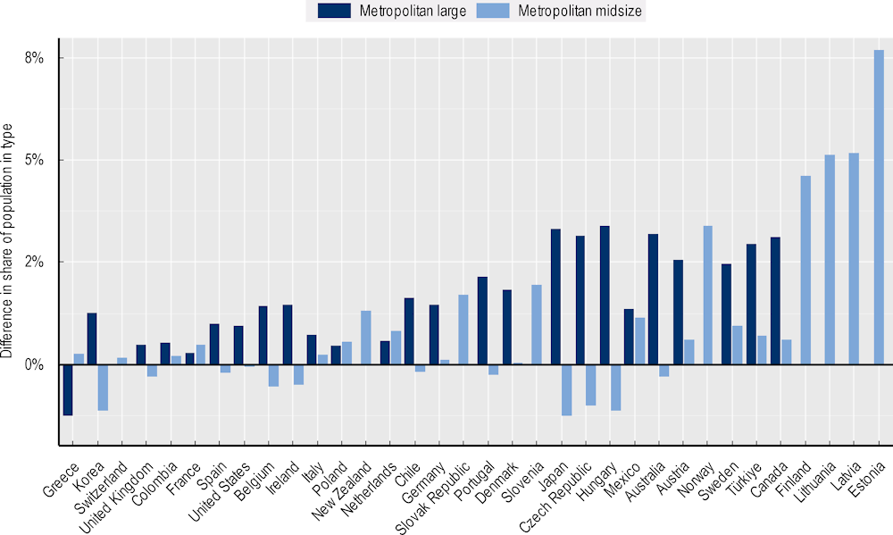
Metropolitan regions host a larger proportion of people today compared to two decades ago in all OECD countries except Greece. A key driver behind this change has been the increasing concentration of population in large metropolitan regions, which increased their population share from around 40% in 2001 to 42% in 2021 (across 24 OECD countries with at least 1 large metropolitan region). Meanwhile, the share of metropolitan midsize regions and remote regions decreased slightly (by 0.3 percentage points), while the share of regions near midsize/large FUAs showed the largest decrease (0.7 percentage points) followed by regions near a small FUA (0.5 percentage points). Within regions, from 2000 to 2015, the share of population living in cities (as defined by the degree of urbanisation) increased by around 3 percentage points across the OECD while the share of population in rural areas decreased.
About half of the countries where the share of population in large metropolitan regions increased saw a decrease in the share of people living in midsize metropolitan regions in 2001-21 (Figure 2.1). Population growth has concentrated in the largest FUAs while about one-quarter of all FUAs in OECD countries are shrinking (see Box 2.1). The increase in the contribution of metropolitan regions is especially large, for example, in small countries with one to three midsize metropolitan regions and no large metropolitan regions (Estonia, Finland, Latvia, Lithuania, the Slovak Republic and Slovenia).
The increasing importance of metropolitan regions results from the compounded effect of internal and international migration and natural growth rates (the difference between births and deaths). Across 28 OECD countries with available data, 29 million people (about 3% of the OECD population) changed their region of residence every, year on average in 2016-19. In that period, metropolitan regions and regions close to them gained respectively 10.5 and 7 persons per every 10 000, while regions far from midsize/large FUAs lost 10 persons for every 10 000 (OECD, 2022[36]). The foreign-born population living in OECD countries reached 138 million in 2021 (10.6% of the total population of OECD countries) (OECD, 2022[37]). Both nationals (and especially youth) and international migrants settle disproportionally in metropolitan areas, especially large ones: 8 in 10 migrants live in metropolitan areas compared to 7 in 10 natives (OECD, 2022[36]) (Table 2.1). Migration, therefore, has made metropolitan regions not only larger but also more diverse and younger (OECD, 2022[38]).
Figure 2.1. Change in share of population in metropolitan TL3 regions, 2001-21
Source: OECD (2022[33]), OECD Regional Statistics (database), https://www.oecd.org/regional/regional-statistics/.
Regions that do not manage to attract working-age migrants eventually see their working-age population shrink and their elderly dependency ratios increase. On average, old-age dependency ratios are higher in non-metropolitan regions (Table 2.1), while remote regions represent the highest share of regions with old‑age dependency ratios above 50% (6.3%, or 46 in 733) compared to other types of regions (5.4% of regions near a midsize/large FUA, 3.5% of regions near a small FUA, 3.4% of metropolitan midsize regions and 1.4% of metropolitan large regions). Furthermore, a larger proportion of non-metropolitan regions is shrinking compared to metropolitan regions: for instance, the proportion of regions that showed shrinking in 2001-21 was 28 percentage points higher in remote regions compared to large metropolitan regions (Table 2.1). Indeed, most regions with the lowest share of working-age population (and high elderly dependency ratios) shrank at a rate of 1% annually or more in the last 2 decades. In Lithuania, Latvia and Portugal, the top three countries facing the largest population decline, regions with a negative annual population growth of at least 1% represented respectively 80%, 67% and 12% of all regions.
Box 2.1. Demographic trends in functional urban areas
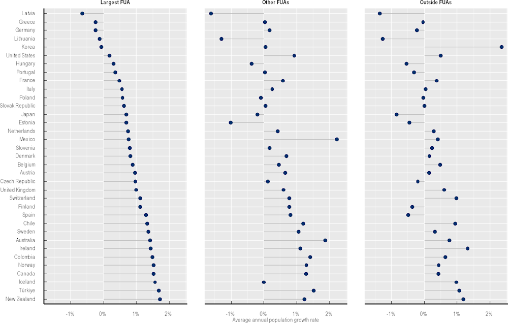
FUAs hosted more than 931 million inhabitants in OECD countries in 2021 (69% of the total population) in 10% of the OECD surface area. Over the last 20 years, the population in FUAs grew on average by 0.7% a year but by only 0.5% in areas outside FUA populations. FUAs’ populations grew in all OECD countries except for Greece, Hungary and Latvia, while the population outside FUAs shrank in ten countries. The largest FUA grew in nearly all OECD countries, except Greece and Latvia (Figure 2.2).
Figure 2.2. Population dynamics in the largest FUA, other FUAs and outside FUAs in OECD countries, 2001-21
Source: OECD (2022[33]), OECD Regional Statistics (database), https://www.oecd.org/regional/regional-statistics/.
Population trends varied with the size of FUAs. FUAs with at least half a million inhabitants had on average the highest annual growth rates (0.71% between 2001 and 2021). FUAs between 250 000 and 500 000 inhabitants had lower growth rates (0.57%) but also lower than FUAs with less than 250 000 inhabitants (0.65%). Furthermore, between 2001 and 2021, 22% of FUAs in OECD countries saw populations shrink. In 11 countries, the share of shrinking FUAs is above 40%.
The tertiary-educated population increasingly concentrates in cities
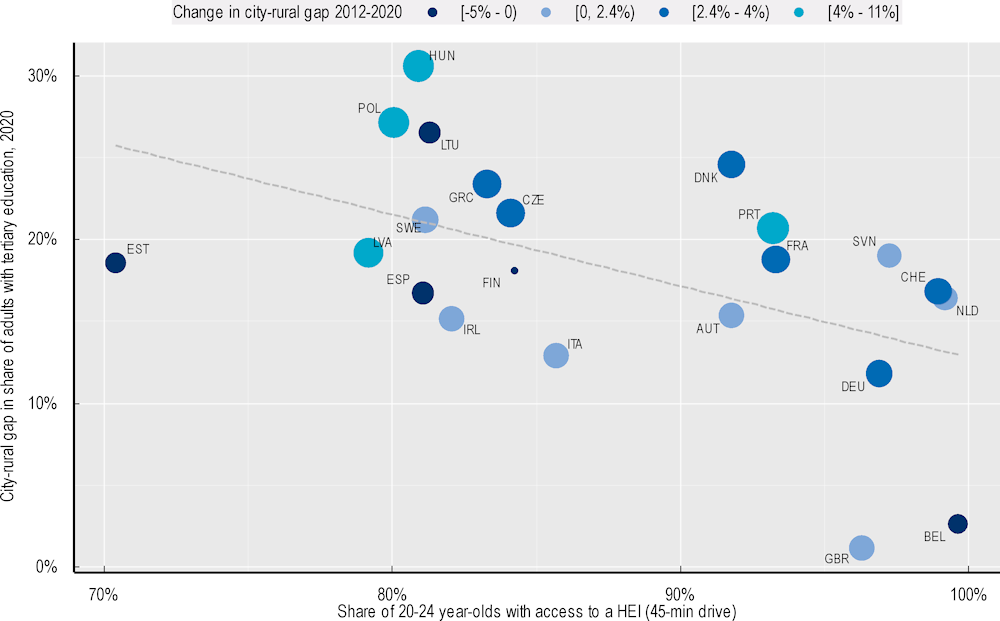
The tertiary educated, i.e. those with a higher education degree, are increasingly concentrated in cities. In 2020, the share of adults with tertiary education was larger in cities than in rural areas in all OECD countries with available data except the United Kingdom (25 out of 26 countries) (Figure 2.3). The gap ranged from 30 percentage points in Hungary to 2 percentage points in Belgium. Compared to 2012, this city-rural gap increased in 19 out of 25 countries with available data, with Poland, Portugal and the Slovak Republic registering the largest increases (about 7 percentage points). However, the share of the tertiary educated increased in all countries during the period and, in all countries except for Hungary, the increase in the city-rural gap was smaller than the increase in the share of the tertiary educated.
Figure 2.3. Access to a higher education institution (20-24 year-olds) versus city-rural gap in the share of tertiary educated (24-65 year-olds), 2012-20
Note: HEI: Higher education institution.
Data only include European OECD countries and the United Kingdom. Tertiary educated status is based on the highest education level attained (ISCED 5-8). Data for main campuses only for Denmark. HEI data for 2020 or the latest year available.
Source: Eurostat (2022[39]), European Union Labour Force Survey, https://ec.europa.eu/eurostat/web/microdata/european-union-labour-force-survey; OECD (2022[40]), “ADHEP database”, Unpublished, OECD, Paris; Mapbox (2022[41]), Navigation, https://docs.mapbox.com/api/navigation/.
People with tertiary education are disproportionally represented in capital city regions in most OECD countries: large capital regions have the highest share of 24-65 year-olds who completed tertiary education in 28 out of 34 OECD countries and accession candidates (i.e. Brazil, Bulgaria, Croatia, Peru and Romania) with available data in 2021 (OECD, 2022[42]). Capital regions can be particularly attractive for the highly educated when they concentrate most of the quality higher education opportunities and a large public sector. However, as discussed in more detail below, they also exhibited the highest income inequalities in half of the 26 OECD countries with available data based on the S80/S20 ratio1 for the disposable income indicator (OECD, 2022[36]).
Rural-urban differences in the share of people with tertiary education may be related to gaps in access to higher education. In 31 OECD countries with available data, 66% of people living in remote regions can access a higher education institution within a 45-minute car trip, compared to 98% for those living in a large metropolitan region. This metric however does not consider the availability and reliability of other means of transportation such as public transport which, when insufficient, can drastically worsen matters, especially for low-income vocational students (OECD, 2022[43]).
Smaller gaps in enrolment in higher education compared to gaps in the share of residents with a higher education degree may point to higher “brain circulation” (i.e. the movement of people for educational purposes). People may get their education outside cities but move to cities in search of quality jobs for professionals. Large city-rural gaps in countries with low access to higher education establishments like Hungary may be related to both poorer access to higher education and lower matching opportunities for professionals outside cities. In contrast, in countries with high access like Portugal, gaps may be mostly related to the concentration of job opportunities in cities (Figure 2.3). Large gaps in the quality of educational offers may not only make the educational offer outside cities less attractive but also lead to worse entrepreneurial or job market outcomes for graduates in rural areas (OECD, 2022[44]; 2022[45]). This may in turn hamper the movement of the tertiary educated to rural areas in search of natural amenities, social and family connections and better housing options.
Establishing evidence of “brain drain” – the increasing flows of educated people from rural areas to cities – nevertheless requires following people over the course of their lives. One of the few studies using cohort data on place of residency versus place of origin of graduates shows that major cities gain and rural areas lose graduates in the United Kingdom, with London consolidated as the main magnet for graduates (Institute for Fiscal Studies, 2021[46]).
Persistent subnational gaps in access to services perpetuate territorial differences in well-being
Available evidence points to substantial subnational gaps in access to services. In OECD countries, travel time, using motorised vehicles, for people living in remote rural areas to reach a healthcare facility is five times longer than those in metropolitan regions. In Europe, students in remote rural areas have to travel on average five additional kilometres to reach a school compared to students in other areas (JRC, 2022[47]).
These gaps may translate into unequal outcomes. Results from PISA2 show that students in city schools obtained higher scores in reading than their peers in schools located elsewhere in all but two OECD countries with available data (OECD, 2022[14]). Moreover, the importance of enhanced access to rural residents may also be greater. For instance, close to one in three rural residents reported suffering from health problems that prevent them from doing things people their age normally do compared to only one in four city residents (OECD/EC, 2020[48]).
Rural facilities are often required to centralise services and keep minimum quality requirements. In healthcare, for instance, rural facilities often face higher relative costs, lower volumes, poorer overall quality and workforce shortages. Across OECD countries, the number of hospital beds per capita in remote regions fell at an average rate of -0.7% per year since the 2008 GFC, while they slightly increased in metropolitan regions (OECD, 2021[11]). The gap in hospital bed rates between metropolitan regions compared to regions far from metropolitan areas – which stood at 50% in 2020 – increased by 5 percentage points with respect to the pre-pandemic period, because hospital bed rates increased faster in metropolitan regions than in regions far from metropolitan areas (18% vs. 14%) (OECD, 2022[36]). The negative impacts on the distance to care (Hsia et al., 2012[49]) and treatment delays for patients due to hospital closures in rural areas can offset any cost gains, especially in the face of sudden increases in demand for care, like during the COVID-19 pandemic (OECD, 2021[11]; 2020[50]).
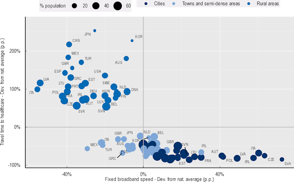
While digital provision offers a way to overcome long travel times, lower economies of scale, longer ambulance transportation times and fewer healthcare workers, rural areas that stand the most to benefit from telemedicine often have poor Internet connectivity levels (OECD, 2021[51]; 2021[11]). Data from regulators in 26 OECD countries indicate a persistent rural-urban divide in connectivity speeds: 1 in 3 households in rural areas do not have access to high-speed broadband on average and, in only 7 out of 26 OECD countries, more than 80% of households in rural regions have access to a high-speed connection (OECD, 2020[52]). Across OECD countries, rural areas facing long travel times to healthcare facilities also face below-average access to high-speed broadband: for instance, in Canada and Mexico, people in rural areas face about 200 percentage points longer travel times and about 40 percentage points fewer Internet speeds than the national average.
Figure 2.4. Location gap in travel time to healthcare versus location gap on Internet speed, OECD countries, 2020
Note: Travel time to healthcare is calculated using driving as a transport mode. Deviation from the national average is calculated from median values by the degree of urbanisation weighted by population levels in each 1 km2 grid cell.
Speedtest data correspond to 2020Q4. The data for average fixed and mobile broadband download Speedtests reported by Ookla measure the sustained peak throughput achieved by users of the network. Measurements are based on self-administered tests by users, carried over iOS and mobile devices. Aggregation according to the degree of urbanisation was based on Global Human Settlement Model (GHS-SMOD) layer grids. The figure presents average peak speed tests, weighted by the number of tests.
Source: For travel time to healthcare: Calculations based on Weiss, D. et al. (2020[53]), “Global maps of travel time to healthcare facilities”, https://doi.org/10.1038/s41591-020-1059-1. For fixed broadband speed: Calculations based on Speedtest® by Ookla® Global Fixed and Mobile Network Performance Maps. Based on analysis by Ookla of Speedtest Intelligence® data for 2020Q4. Provided by Ookla and accessed 2021‑01‑27 (see OECD (2021[51]) for details). Ookla trademarks are used under license and reprinted with permission.
Regional inequalities will evolve in a context of a shrinking population in half of OECD countries
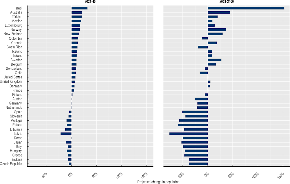
In the medium and long terms, changes in the distribution of people within countries will happen in the context of stable or decreasing population stocks in half of OECD countries. Populations are expected to decline in 14 OECD countries by 2040 and 18 by 2100, with the largest decreases in East and Southern European countries, Japan and Korea (Vollset et al., 2020[54]). Besides differences in fertility rates – which were already below replacement levels in all OECD countries except Israel in 2021 – differences in international migration and life expectancy drive differences in projected population changes.
The future also holds fundamental changes in age structures across OECD countries: the number of children under 5 years of age could decline from 63.5 million in 2021 to about 59.2 million in 2040 whilst the number of elderly (older than 80 years) is expected to nearly double, from 66.5 million to 114.7 million (Vollset et al., 2020[54]). These population projections have stark implications for elderly dependency ratios in OECD countries: while in 2021, there are about 13 working-age people (15-64 years old) for every elderly person, in 2040, there will be only 7 (Rouzet et al., 2019[55]; OECD, 2019[56]; 2022[14]).
Figure 2.5. Medium- and long-term population projections, OECD countries, 2021-2100
Note: Change is calculated as the difference between years over the initial value.
Source: Based on data from Vollset, S. et al. (2020[54]), “Fertility, mortality, migration, and population scenarios for 195 countries and territories from 2017 to 2100: A forecasting analysis for the Global Burden of Disease Study”, https://doi.org/10.1016/s0140-6736(20)30677-2.
Against this backdrop, metropolitan regions are expected to slightly increase their population share by 2040. In absolute terms, the number of people living in metropolitan regions is expected to remain constant by 2040, while the number of people in non-metropolitan regions is expected to shrink (by 2.8% and 2.3% in regions near and far from a midsize/large FUA) (OECD, 2022[36]).
Within regions, the population living in FUAs in OECD countries is expected to increase from 950 million to 1 billion. Most of this increase will concentrate in large FUAs, which are expected to grow by 5% by 2030 while small and medium-sized FUAs are expected to shrink by 4% and 3% over the same period (OECD, 2022[36]). Areas outside cities are also projected to increase in absolute terms but at a slower pace than cities. By 2050, the population in towns and semi-dense areas is projected to increase from 2.1 billion to 2.3 billion worldwide, while the population in rural areas is expected to expand from 1.7 billion to 1.9 billion (OECD/EC, 2020[48]).
Regional income inequality: Past, present and future outlook
The evolution of regional income inequalities3 hinges upon both the relative evolution of national income per capita levels (linked to national GDP per capita growth) and the redistribution of income within countries. Major economic shocks have an effect not only on national growth rates but also on gaps in income per capita across regions. This is because regions differ in their degree of resilience to shifts and shocks (Rice and Venables, 2020[57]). Structural factors then – and in particular the resilience of those factors to shocks – rather than shocks per se are key drivers of regional inequalities (Garcilazo, Moreno-Monroy and Oliveira Martins, 2021[58]; OECD, 2022[59]).
The 2008 GFC put a halt to regional convergence in many OECD countries (OECD, 2022[36]; 2020[16]; Faggian and Ascani, 2021[60]). In this context, the income gaps between metropolitan and non-metropolitan regions have not closed since then, in part because metropolitan regions have proven to be more resilient to crises than non-metropolitan regions (OECD, 2020[16]). In the past two decades, the gap between GDP per capita in non-metropolitan versus metropolitan regions – of around 68% – did not close across the OECD (OECD, 2022[36]).
This section presents evidence of regional income inequality trends. It focuses mostly on small (TL3) regions in 2000-20, which offer a more granular territorial analysis and allows for classifications based on access to cities (see Annex 2.A). This section does not attempt to draw inferences regarding the effect of the COVID-19 pandemic as current data available (2019-20) are not sufficient to evaluate the impact of and recovery from this shock on regional income inequalities. The section starts by proposing a classification of OECD countries according to their regional income inequality trends. It then identifies distinct growth inequality paths. The section then assesses the importance of metropolitan versus non‑metropolitan gaps in driving regional income inequalities across countries. Finally, it explores the role of proximity between regions in driving regional income inequality.
The data used in the analysis have several limitations (see also Annex 2.A). This section assesses differences in income inequalities across regions and FUAs, which reflect underlying structural, including geographical, factors as well as demographic differences (e.g. higher elderly dependency ratios). Whilst there is also interest in identifying spatial differences in income inequalities for similar demographic cohorts (e.g. gender, age, race and sexual orientation), data to assess these are unfortunately unavailable (see Box 2.2).4 As data on disposable income are unfortunately not available for small regions, the section uses regional GDP per capita as a proxy for the typical income of a representative individual in a region (this interpretation applies to the unweighted version of the Theil index, see Gluschenko (2017[61])). This means that the regional inequality measures used in this section are not indicative of the evolution of inter-personal inequalities or the situation of any given income-group (Rey, Arribas-Bel and Wolf, 2020[62]).
Box 2.2. Bottom-up versus top-down approaches to measuring regional income inequality
A top-down approach allows for high frequency and large country coverage but has several shortcomings
International comparative measures of spatial income inequality aim at capturing to what extent people of different incomes live in different locations. Locations can vary in levels of spatial aggregation, from large areas such as countries to small areas such as neighbourhoods. A “top-down” approach to measuring regional income inequality over time, which this chapter uses, is to combine GDP (“income”) with population counts series.
Aggregated series allow for the identification of trends across many countries because they are available in most OECD countries, are comparable across countries and are available yearly. However, they have several shortcomings: i) GDP and population may not be recorded in the same place, requiring further aggregation (e.g. of all small regions that are part of the same FUA, see Annex 2.A); ii) in countries with significant shares of capital-intensive industries (e.g. mining), GDP per capita levels likely do not reflect the income levels of the average resident; iii) aggregate series do not provide insights on the full income distribution within regions (see Annex 2.A for further explanation); iv) residents in one region may work in another region, thus contributing to the GDP per capita of that region but contributing directly to their own income, which means that translating differences in GDP per capita levels across regions (that provide important insights on broader economic growth, including on fiscal potential of regions) to assess differences in the disposable income of residents should be done with care.
A bottom-up approach is preferable for understanding household personal incomes and allows to look at different parts of the income distribution but is not available for a wide number of countries and years
A “bottom-up” approach uses declared incomes and location information available from administrative sources, primarily tax records. This approach allows for measuring income disparities across regions as well as income inequality within regions.
The main advantages of this approach compared to a “top-down” one includes: the availability of information on the full income distribution, as opposed to mean levels only; high geographical granularity (going even below the small region level); and more accuracy in definitions to capture more precisely the disposable income of households. However, the main drawbacks of this approach are in turn its relative infrequency (e.g. by census rounds, every 5 or 10 years) and more difficulties in establishing international comparability, as reported taxable units (e.g. households or individuals) and types of income (e.g. gross or disposable) vary across countries.
Recent OECD work (Königs et al., forthcoming[63]) uses administrative records to analyse income levels and distributions for small regions (TL3) and smaller units (e.g. municipalities) in half of OECD countries. However, these data are only available for a relatively short time span – in most cases starting in the mid-2000s – which limited the study of regional income inequality to current trends rather than to long‑term dynamics. The main findings align with those of this chapter:
Trends in regional income disparities are not uniform across countries, but regional median incomes have converged over the last decade in most of the countries with available data.
Income disparities between regions account for a very small fraction of overall income inequality. Instead, disparities within the same region account for at least 95% of the overall inequality.
Regional income disparities are high in some countries. Across small (TL3) regions, median household incomes for the highest- and lowest-income regions differ by a factor of only 1.2 to 1.3 in some of the Nordic countries, but by 1.7 and 1.6 in Japan and Latvia.
Metropolitan regions concentrate on high median incomes and high inequalities. Across 17 countries with available data, over 75% of large metropolitan regions are in the top quartile of regions by median income and by the level of inequality.
Source: Königs, S. et al. (forthcoming[63]), “The geography of income inequalities in OECD countries: Evidence from national register data”, OECD Publishing, Paris.
Income per capita gaps have narrowed between OECD countries but gaps within countries remain large
Over the last two decades, most OECD regions have seen improvements in their GDP per capita ratios but with significant divergences between small regions at the top and bottom of the income distribution. Top concentration and divergence of bottom regions persisted during the period, except in 2020 for the first year of the COVID-19 pandemic, leading in turn to an increase in the mean-to-median ratio5 (Figure 2.6, Panel B; see Table 2.2).
The structural effects of COVID-19 on regional inequalities will take time to materialise and, as such, it is not yet possible to interpret the impact of the pandemic on bottom convergence and top deconcentration observed in 2019-20 as a new trend of declining inequalities or a temporary consequence of the fall in economic activity during that period.
Table 2.2. Summary of main concepts related to regional income inequality
|
Concept |
Definition |
Measurement |
|---|---|---|
|
Increase/decrease in income per capita regional inequality |
Increase/decrease in the Theil index or mean-to-median ratio |
Unweighted Theil index of TL2/TL3 GDP per capita; mean TL2/TL3 GDP per capita over median TL2/TL3 GDP per capita |
|
Top concentration/deconcentration |
Increase/decrease in the top 20% to mean ratio |
Mean GDP per capita in top 20% regions over mean TL3 GDP per capita in a given year |
|
Bottom regions convergence/divergence |
Increase/decrease in the bottom 20% to mean ratio |
Mean TL3 GDP per capita in bottom 20% regions over mean TL3 GDP per capita in a given year |
|
Polarisation/depolarisation |
Increase/decrease in the top 20% to bottom 20% ratio |
Mean TL3 GDP per capita in the bottom 20% of regions over mean TL3 GDP per capita in the top 20% of regions |
|
Between (group) inequality |
Variability across the group (i.e. country) means with respect to the overall (OECD) income per capita mean |
Theil index between/within decomposition based on TL2/TL3 GDP per capita (see Annex C in OECD (2020[52])) |
|
Within (group) inequality |
Variability in regional income per capita with respect to their group mean |
Note: Top/bottom calculated as population equivalent (top/bottom regions with at least 20% of the population). The interpretation of top/bottom 20% GDP per capita is that 20% of the population in the country holds 20% of the value.
Source: Based on multiple sources.
The Theil index offers a way to observe the variability of regional incomes per capita in OECD countries in a single measure. The index compares the income per capita in each region to the mean of all regions across OECD countries. The index partly captures differences in GDP per capita levels across countries: for instance, if a country experienced faster growth than the OECD average each year while everything else remained the same, the Theil index would decrease, even though the variation in regional incomes stayed the same. The index decomposition into a “between” and a “within” component is useful to assess the changes in the variability of regional income per capita, controlling for the effect of changes in national income per capita (see Box 2.3 and Table 2.2) (OECD, 2020[52]; Elbers et al., 2008[64]).
Figure 2.6. Trends in GDP per capita inequality indicators, TL3 OECD regions, 2000-20
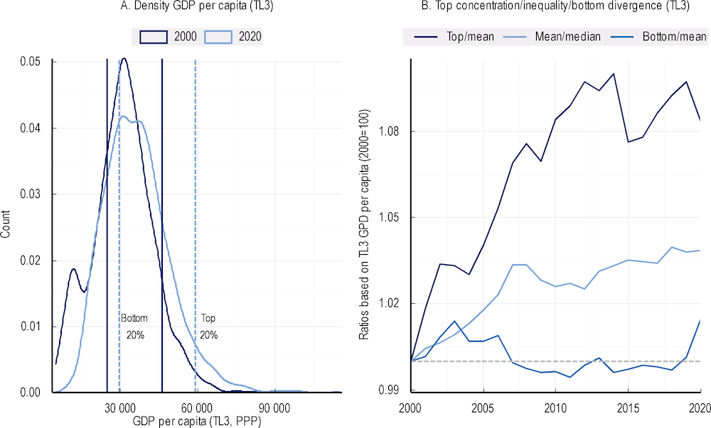
Note: Vertical lines in Panel B represent group mean values.
The density GDP per capita plot does not include 4 TL3 regions with GDP per capita over EUR 150 000. Based on 26 OECD countries with available GDP per capita data for 2000-20 and more than 1 TL3 region.
Source: OECD (2022[33]), OECD Regional Statistics (database), https://www.oecd.org/regional/regional-statistics/.
Box 2.3. Theil index of regional inequality and its decomposition
Decomposition of the Theil index
The Theil index of regional income inequality measures the spread (variance) in GDP per capita levels across regions. It is the sum of the (log) ratio of GDP per capita in region and the mean GDP per capita over all regions, weighted by the share of region in the total GDP per capita:
with
The assumption when applying the Theil index to regional inequality is that each region is composed of a representative individual with an income approximated by the average GDP per capita of their region and, therefore, the index is invariant to how many people live in each region but not to the number of regions there are in the country.
Standard between/within decomposition of the Theil index
The Theil index for regional inequality can be further refined to capture the contribution within specific groups (e.g. countries) and between those groups. To determine the “between” contribution, we take the sum of the (log) ratio of the average GDP per capita in each group and the mean GDP per capital over all regions, weighted by the share of GDP per capita of group in total GDP per capita:
with
To determine the “within” contribution, we calculate the inequality in regional incomes with respect to their group means, weighted by the share in their group and the share of their group in the total (equal to the share of GDP per capita of the region in the sum of total GDP per capita):
Separating country-level convergence (between) from region-level convergence (within) is of particular relevance, not least because the evidence does point to a “catching-up” effect in many countries, particularly former industrial transition economies in the European Union, Korea and Türkiye. Ten out of 13 countries with GDP per capita below OECD averages in 2000 saw the gaps narrow in the last 2 decades (Figure 2.7). On the other hand, some countries, notably Greece, Italy, Portugal and Spain saw gaps grow relative to the OECD average. Overall, 19% of the OECD population lived in regions within countries experiencing upwards convergence and 12% lived in countries experiencing divergence.
Figure 2.7. Country GDP per capita gap with respect to OECD mean, 2000 and 2020
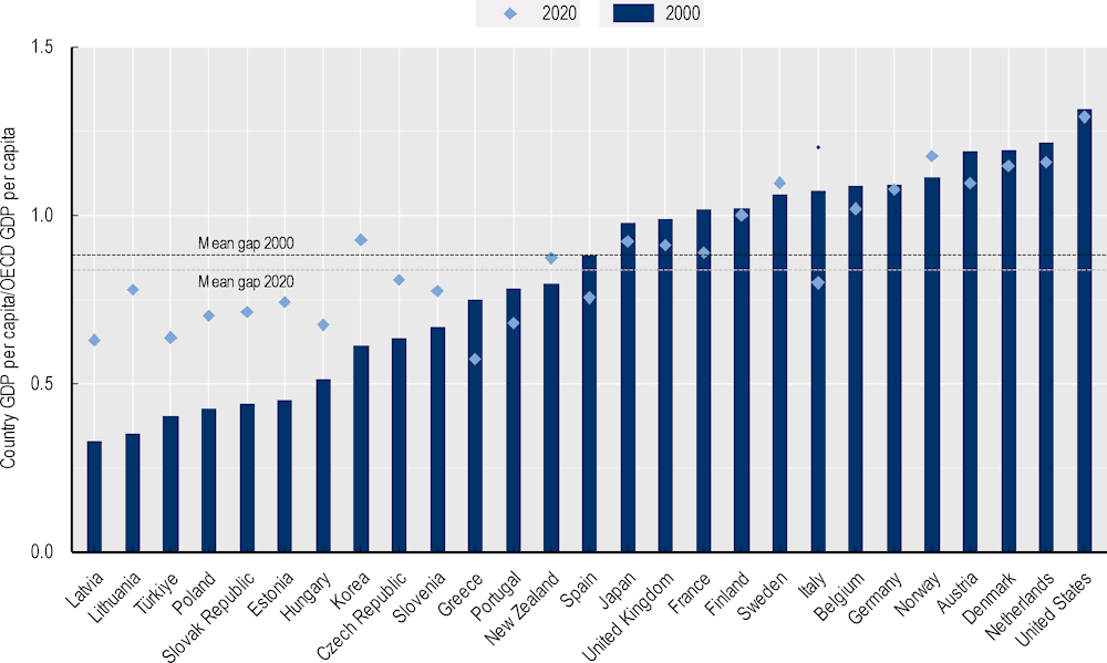
Note: Based on country aggregates from TL3-level data. The gap is defined as each country’s GDP per capita with respect to OECD GDP per capita. The mean gap is the mean value of gaps across OECD countries. Converging countries had a 2000 GDP per capita gap below the mean gap across OECD countries and a smaller gap in 2020 (i.e. a larger country GDP per capita to OECD GDP per capita ratio): the Czech Republic, Estonia, Hungary, Korea, Latvia, Lithuania, New Zealand, Poland, the Slovak Republic, Slovenia and Türkiye. Diverging countries had a 2000 GDP per capita gap in below the mean gap across countries and a larger gap in 2020 (i.e. a smaller country GDP per capita to OECD GDP per capita ratio): Greece, Italy, Portugal and Spain. Countries above OECD levels had gaps above the mean gap across OECD countries in 2000 and 2020: Austria, Belgium, Denmark, France, Finland, Germany, Japan, the Netherlands, Norway, Sweden, the United Kingdom and the United States.
Source: OECD (2022[33]), OECD Regional Statistics (database), https://www.oecd.org/regional/regional-statistics/.
The broad convergence in overall between-country inequalities capture in Figure 2.7 is also reflected in the Theil “between” measure (see also Box 2.3) in Figure 2.8. However, whilst inequalities between countries have, on the whole, declined over the last two decades, this has not been mirrored with similar progress on within-country inequalities. At the large region (TL2) level for example, within-country inequalities increased from 2000 to 2015 before decreasing, while at the small region (TL3) level, within-country income inequalities slightly increased over the period, with marginal improvements often occurring during severe economic shocks. The absolute levels of within-country inequality stayed in a narrow range compared to changes in between-country inequality, so decreasing between-country inequality drove decreases in overall inequality across large and small regions. In both cases, the decrease in between-country inequality compensated for the rise in within-country inequality.6
Figure 2.8. Trends in total, within and between regional income inequality TL2 and TL3 OECD regions, 2000-20
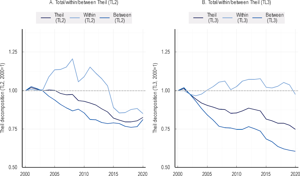
Note: Panel A is based on 385 TL2 regions in 28 OECD countries with available data (no TL2 data [continuous time series for more than 1 region] available for Chile, Costa Rica, Estonia, Iceland, Israel, Ireland, Latvia, Lithuania, Luxembourg and Switzerland). Panel B is based on 1 586 TL3 regions in 27 countries with available data (no TL3 data [continuous time series for more than 1 region] for Australia, Canada, Chile, Colombia, Costa Rica, Iceland, Ireland, Israel, Luxembourg, Mexico and Switzerland). Between Theil measures the dissimilarity of the national GDP per capita means with respect to the OECD average. Within Theil measures the dissimilarity between regional and national GDP per capita. See Box 2.3 more for details.
Source: OECD (2022[33]), OECD Regional Statistics (database), https://www.oecd.org/regional/regional-statistics/.
Over half of OECD countries saw regional income inequalities increase in the last two decades
Looking only at regional inequalities among small regions (TL3), 15 out of 27 countries with available data since 2000 saw regional income inequalities increase over the last 2 decades (Table 2.3) (see Annex Table 2.B.1 for the full set of results). This means that 70% of the OECD population live in countries (with available data) that experienced increases in regional income inequality. Table 2.3 also differentiates countries on whether they were converging to or diverging from the OECD average (see also Figure 2.7) and further classifies countries on the basis of weather their Theil index followed a mostly linear (increasing/decreasing) or a non-linear trend (e.g. u-shape or inverted u-shape).
Table 2.3. A typology of regional income inequality trends based on GDP per capita at the TL3 level
|
Broad type |
Detailed type |
At/above mean OECD GDP per capita gap (period max; period min) |
Converging to OECD GDP per capita (period max; period min) |
Diverging from OECD GDP per capita (period max; period min) |
|---|---|---|---|---|
|
Income inequalities mostly increasing over the period |
Linear |
Belgium (2003-05; 2000-02), Denmark (2015-18; 2000-02), France (2018-20; 2003-05), Sweden (2018-20; 2003-05), United Kingdom (2018-20; 2003‑05) |
Estonia (2015-17; 2006-08) |
Italy (2018-20; 2006-08) |
|
Non-linear |
Japan (2006-08; 2000-02), United States (2012-14; 2000-02) |
Czech Republic (2018-20; 2000-02), Hungary (2009-11; 2000-02), Lithuania (2006-08; 2000-02), Poland (2015-17; 2000-02), Slovak Republic (2009-12; 2000‑02), Slovenia (2009-11; 2000-02), |
|
|
|
Income inequalities mostly decreasing over the period |
Linear |
Finland (2000-02; 2018-20), Norway (2000-02; 2018-20) |
Latvia (2003-05; 2009-11), Türkiye (2006-08; 2015-17) |
Greece (2006-08; 2015-17), Portugal (2000-02; 2018-20) |
|
Non-linear |
Austria (2006-08; 2018-20), Germany (2000-02; 2018-20), Netherlands (2000-02; 2018-20) |
Korea (2009-12; 2018-20), New Zealand (2009-11; 2018-20) |
Spain (2000-02; 2009-11) |
Note: See Annex 2.B for details. Linear/non-linear trend determined based on the sign and statistical significance (95% confidence level) of the coefficients of a regression of the second-degree polynomial of the Theil index against time. Decreasing/increasing determined according to the sign of the compounded growth rate of the Theil index between 2000-02 and 2018-20. Converging countries had a 2000 GDP per capita gap below the mean gap across OECD countries and a smaller gap in 2020 (i.e. a larger country GDP per capita to OECD GDP per capita ratio). Diverging countries had a 2000 GDP per capita gap below the mean gap across countries and a larger gap in 2020 (i.e. a smaller country GDP per capita to OECD GDP per capita ratio). The gap is defined as each country’s GDP per capita with respect to OECD GDP per capita. The mean gap is the mean value of gaps across OECD countries.
Source: Based on data from OECD (2022[33]), OECD Regional Statistics (database), https://www.oecd.org/regional/regional-statistics/.
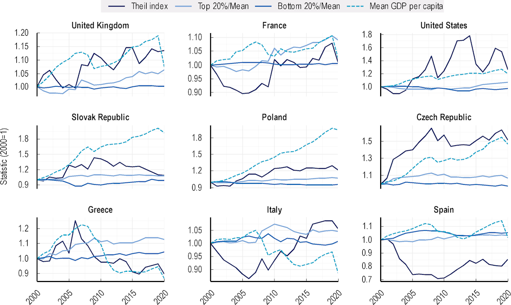
Table 2.3 reveals that beyond the general picture, there are different growth-inequality trajectories across OECD countries, confirming there is no single narrative on regional income inequalities (McCann, 2022[65]) (Figure 2.9). Rather, while most OECD countries that showed increasing inequality in the last two decades reached their minimum values of regional GDP per capita inequality before the GFC, they were then set on different trajectories.
On the one hand, among OECD countries with income per capita above OECD levels, some such as France and the United Kingdom, experienced a sustained increase in regional inequality since the mid-2000s, while others, such as Germany and Portugal, saw sustained falls.
On the other hand, virtually all countries converging towards OECD GDP per capita levels saw within-country inequalities rise over the period as a whole but in a non-linear fashion (mostly as an inverse U). In Poland for instance, inequality started picking up in 2004 and continued increasing until 2020. In Hungary and the Slovak Republic, inequalities also increased rapidly, albeit from relatively low levels, between 2003/04 and 2009, but unlike Poland, fell between 2010 and 2020. In the Czech Republic, Estonia and Lithuania, inequalities plateaued at relatively high levels after decreasing slightly from their peaks in the aftermath of the GFC in 2010.
In most countries, increasing regional inequality went hand in hand with bottom divergence and top concentration (and vice versa, decreasing inequality went hand in hand with bottom convergence and top deconcentration). The correlation between changes in the Theil index and the top-to-mean (bottom-to-mean) was above (below) 0.7 in 21 (22) countries out of 27 with available data. Exceptions include the Czech Republic, Norway and the United Kingdom, which all showed a weak correlation between inequality and bottom region trends but a strong correlation with respect to top concentration.
Figure 2.9. Trends in GDP per capita inequality indicators for selected countries, TL3 regions, 2000‑20
Source: OECD (2022[33]), OECD Regional Statistics (database), https://www.oecd.org/regional/regional-statistics/.
Growth-inequality paths were counter-cyclical in most countries with declining regional inequality, and pro‑cyclical in most countries with increasing regional inequality (Figure 2.10, Panel C). In some cases, including France, Italy and Spain, the pattern switched from counter-cyclical to pro-cyclical after the GFC, in line with findings that the GFC put a stop to regional convergence in these countries (Diemer et al., 2022[17]; OECD, 2020[16]). Greece is the only country with a pro-cyclical growth-inequality trend, as the Theil index closely followed the decreasing trend in GDP per capita in the last two decades.
Figure 2.10. Correlation between the Theil index of TL3 GDP per capita with top-to-mean and bottom-to-mean ratios and mean GDP per capita, 2000-20
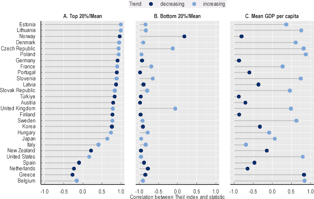
Note: Increasing/decreasing trends follow classification in Table 2.3.
Top/bottom calculated as population equivalent (top/bottom regions with at least 20% of the population). The interpretation of top/bottom 20% GDP per capita is that 20% of the population in the country holds 20% of the value.
Source: OECD (2022[33]), OECD Regional Statistics (database), https://www.oecd.org/regional/regional-statistics/.
Gaps between top and bottom regions did not narrow in most OECD countries over the last two decades
Polarisation increased in 14 out of 27 OECD countries with available data. Despite decreases in the last two decades, the ratio of top to bottom region in 2020 was still the highest in Türkiye (3.2), followed by the Slovak Republic (2.9) and Poland (2.8).7 Absolute gaps in top versus bottom region incomes however increased in the majority (21 out of 27) of OECD countries with available data in 2010-20 compared to 2000-09 (OECD, 2022[59]) (Figure 2.11, Panel B), including in countries such as Germany, Hungary, Latvia and Türkiye where the relative gaps decreased. Reducing polarisation in both relative and absolute terms requires necessarily that bottom regions grow faster than top regions. In the case of Latvia, for instance, bottom regions would have needed to grow twice as fast as they did between 2000 and 2020, just to maintain the same absolute gap over time.
The evidence on increasing polarisation at the small region level is consistent with findings for disposable income at the large region level. Disposable income and poverty rates differ substantially across OECD countries and within their large regions. In 2020, 11 out of 26 OECD countries with available data had regions with S80/S20 ratios above the OECD average, including most regions in Chile, Colombia, Mexico and the United States. Moreover, the average gap in poverty rates between the worst- and best-performing regions in the same country was 18 percentage points, reaching 50 percentage points in Colombia and Mexico (OECD, 2022[36]).
Figure 2.11. Relative vs. absolute changes in polarisation based on real GDP per capita, TL3 OECD regions, 2000-20
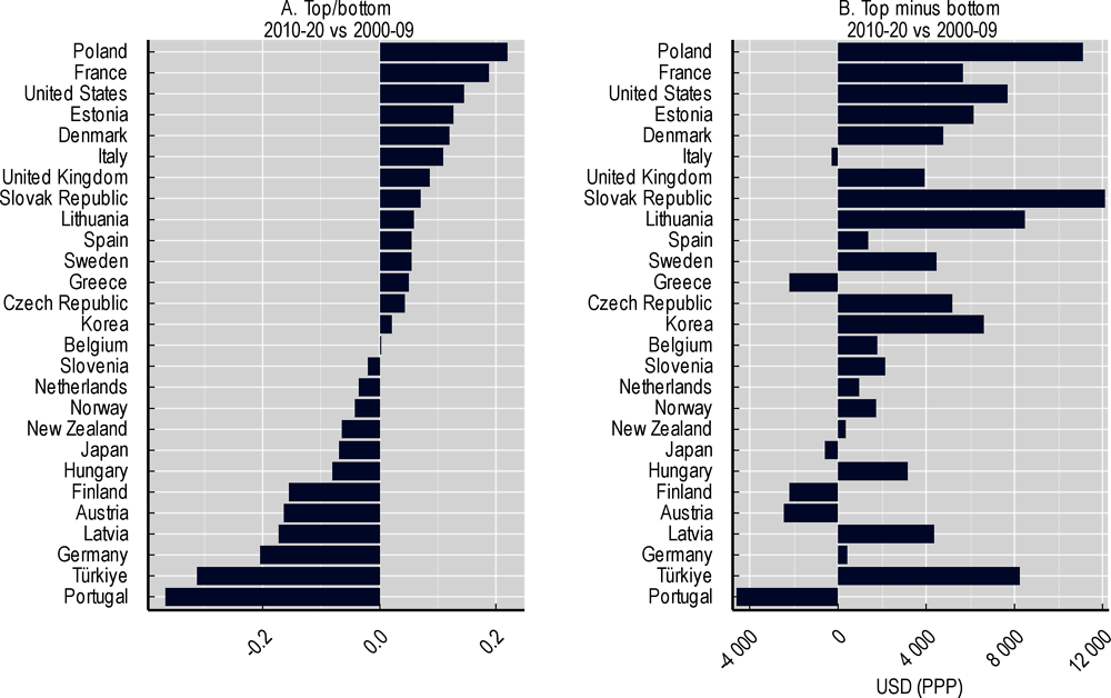
Note: Top/bottom calculated as population equivalent (top/bottom regions with at least 20% of the population). The interpretation of top/bottom 20% GDP per capita is that 20% of the population in the country holds 20% of the value.
Source: OECD (2022[33]), OECD Regional Statistics (database), https://www.oecd.org/regional/regional-statistics/.
Differences in income per capita between metropolitan/top and other regions drive regional income inequalities in most OECD countries
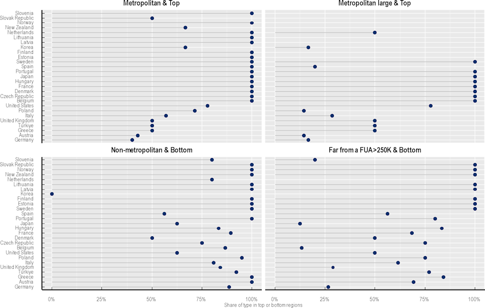
Regional income inequalities have increased because metropolitan regions have continued to pull apart from other regions in a majority of countries. A decomposition of the Theil index of inequality can shed light on whether differences between metropolitan and other regions matter the most for regional income inequality and whether distance to cities has a role in explaining regional income inequalities (see Box 2.4, (Elbers et al., 2008[64]; Boulant, Brezzi and Veneri, 2016[66]). At the same time, polarisation and bottom divergence are linked to metropolitan versus non-metropolitan gaps because a significant share of top (bottom) regions are metropolitan (non-metropolitan). Proximity to large FUAs is also an important factor: for instance, in some countries all top regions are metropolitan large and in others all bottom regions are far from midsize/large cities (see Box 2.5 for more information on the overlap between top/bottom and metropolitan/non-metropolitan regions).
Box 2.4. A measure to compare the share of between-group inequality across countries
Evaluating observed between-group inequality against a benchmark of maximum between-group inequality
The standard Theil decomposition is sensitive to the number of groups considered. For instance, if one were to consider a split between two categories (e.g. metropolitan versus non-metropolitan), the share of between-group inequality would be very small. As this result is an artefact of the standard Theil decomposition, concluding from this that metropolitan/non-metropolitan differences matter little for regional inequality would be misleading.
Elbers et al. (2008[64]) have proposed a decomposition that normalises the Theil index by the observed number and relative size of observed groups. This decomposition is better suited for comparisons that involve different numbers of group and/or different group shares, so that:
where BGI is Between-Group Inequality. This measure “replaces total inequality in the denominator of the conventional ratio with the maximum between-group inequality that could be obtained if the number of groups and their sizes were restricted to be the same as for the numerator”.
Notes: In the calculations, Rb’ is obtained using the decompGEI function of the R package IC2, available at: https://www.rdocumentation.org/packages/IC2/versions/1.0-1/topics/decompGEI.
The decomposition measures the share of inequality explained by differences between groups of regions. As these shares are sensitive to the number of regions in each country, country values are expressed as a ratio of OECD-wide shares. Table 2.4 classifies countries according to the maximum relative share among three possible groupings (see Annex Table 2.B.2 for full results): i) large metropolitan regions versus other regions; ii) metropolitan versus non-metropolitan regions; and iii) regions far from a midsize/large FUA versus other regions. The table also distinguishes between countries where all (large) metropolitan regions are top regions.
Table 2.4. Contribution of TL3 region types to regional income inequality, based on 2010-20 averages
|
Large metropolitan/top vs. the rest |
Large metropolitan vs. the rest |
Metropolitan/top vs. the rest |
Metropolitan vs. the rest |
Far from a FUA>250K vs. the rest |
|---|---|---|---|---|
|
Czech Republic Denmark France Hungary Portugal Sweden |
Korea Poland Türkiye United Kingdom United States |
Belgium Estonia Finland Latvia Lithuania Netherlands Norway Slovak Republic Spain |
Germany Japan New Zealand Slovenia |
Austria Greece Italy |
Note: Countries with increasing inequality are listed in bold.
Countries selected based on the largest 2010-20 average share of between-group inequality relative to OECD values. See Annex Table 2.B.1 for full results. Far from an FUA>250K includes regions near/with a small FUA and remote regions. Top/bottom calculated as population equivalent (top/bottom regions with at least 20% of the population). The interpretation of top/bottom 20% GDP per capita is that 20% of the population in the country holds 20% of the value.
Source: Based on OECD (2022[33]), OECD Regional Statistics (database), https://www.oecd.org/regional/regional-statistics/.
Concerning metropolitan versus non-metropolitan differences, the size of cities and distance to a city matter to different degrees across countries, leading to different patterns:
The relative differences in the income per capita group of large metropolitan regions and others with respect to OECD levels explain the largest share of regional income inequality in 11 out of 19 countries with large metropolitan regions (8 of which have increasing inequality). In six of these countries, all top regions are also large metropolitan regions.
The relative differences in income per capita in the broader group of metropolitan versus non‑metropolitan regions mattered the most in 13 out of 27 countries with available data. This included five countries with large metropolitan regions (two of which had increasing inequality) and all eight countries with no large metropolitan regions.
Finally, relative differences between regions far from a midsize/large FUA and other regions mattered the most in the three countries (with Italy being the only country in the group with increasing inequality).
Furthermore, comparing changes between 2000-09 and 2010-20 reveals that:
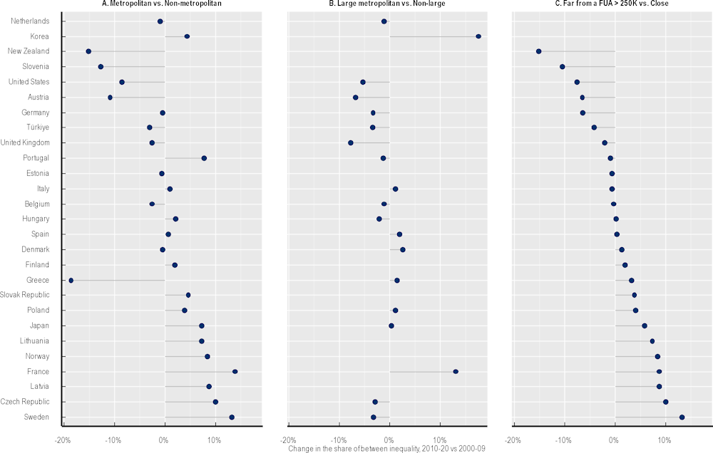
The share of inequality explained by differences between metropolitan and non-metropolitan regions increased in 13 out of 27 OECD countries with available data, 7 of which had increasing inequality (the Czech Republic, France, Hungary, Japan, Latvia, Poland, the Slovak Republic and Sweden) (Figure 2.12). This share did not necessarily increase in all countries where income inequality increased: in 8 countries with increasing inequality, including the United Kingdom and the United States, this share was smaller in 2010-20 compared to 2000-09.
The share of inequality explained by differences between large metropolitan and other regions increased in 8 out of 19 OECD countries with large metropolitan regions. This included three countries with increasing inequality where the other shares considered did not increase (Denmark, Italy and the United Kingdom).
The importance of differences between regions far from cities and others increased in ten OECD countries, six of which had increasing inequalities.
Figure 2.12. Changes in the contribution of region types to regional income inequality based on TL3 GDP per capita, 2000-20
Source: Based on OECD (2022[33]), OECD Regional Statistics (database), https://www.oecd.org/regional/regional-statistics/.
Box 2.5. Overlap between top/bottom and metropolitan/non-metropolitan regions
Regions can be classified according to the Access to Cities typology (see Annex 2.A) or as top or bottom regions. In seven countries (Estonia, Finland, Latvia, Lithuania, Norway, Portugal and Sweden), all top regions are metropolitan and all bottom regions are non-metropolitan. In all of these countries except for Portugal, all bottom regions are far from a midsize/large FUA.1 In four countries, all bottom regions are non-metropolitan (Austria, Greece, New Zealand and the Slovak Republic). In New Zealand and the Slovak Republic, all bottom regions are far from a midsize/large FUA.
The match between metropolitan and top regions on the one hand and non-metropolitan and bottom regions on the other is substantial but not perfect. In nine countries (Belgium, the Czech Republic, Denmark, France, Hungary, Japan, the Netherlands, Slovenia and Spain), all top regions are metropolitan but not all bottom regions are non-metropolitan. In six of these countries (Belgium, the Czech Republic, Denmark, France, Hungary and Japan), all top regions are large metropolitan. Finally, in 5 countries, the overlap between non-metropolitan and bottom regions is larger than the overlap between metropolitan top and top regions: Germany (38% vs. 89%), United Kingdom (80% vs. 50%), Italy (81% vs. 57%), Poland (95% vs. 71%) and Türkiye (92% vs. 50%). In two countries, the opposite is true (United States [78% vs. 63%] and Korea [66% vs. 0%]).
Figure 2.13. Share of top/bottom regions by region type, based on 2020 values for top/bottom regions
Note: Top/bottom calculated as population equivalent (top/bottom regions with at least 20% of the population). The interpretation of top/bottom 20% GDP per capita is that 20% of the population in the country holds 20% of the value.
Source: OECD (2022[33]), OECD Regional Statistics (database), https://www.oecd.org/regional/regional-statistics/.
1. The reminding countries in this group do not have non-metropolitan regions near a metropolitan area.
Differences between clusters of high- and low-income regions drive regional inequalities in many countries
The measures of regional inequality used thus far do not consider the geographical aspect of regions, that is, the fact that regions with similar characteristics may be close or distant to each other (Rey, Arribas-Bel and Wolf, 2020[62]). The spatial Gini index disentangles the effect of proximate versus distant regions in the Gini index (Rey and Smith, 2012[67]). When spatial dependence is high and positive (similar regions show a strong tendency to cluster), differences with distant regions drive inequality, as values are similar among neighbours.
The spatial Gini index for GDP per capita shows that differences across distant regions drive virtually all the variation in regional inequality in large OECD countries including France, Germany and the United States and in countries with high regional divides such as Italy (Figure 2.14). In contrast, in small countries where a large share of inequality is due to concentration in the capital city, there is no evident clustering of regions with high or low income per capita but rather an “oasis” of prosperity.
Figure 2.14. Spatial Gini index of GDP per capita at the TL3 level, OECD countries, 2021
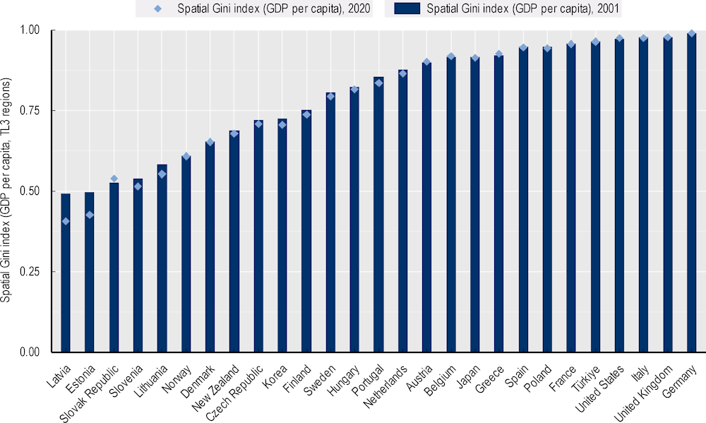
Note: The index measures the share of inequality due to differences between proximate and distant regions.
GDP per capita data are not aggregated by metropolitan regions sharing the same FUA (see Annex 2.A for details). The spatial Gini is equal to the neighbour composition of the Gini coefficient times one over the Gini coefficient (Parry, 2022[68]). The spatial Gini considers the role of proximity in the concentration of a given variable. It decomposes the Gini index into two components: one among neighbours (i.e. nearby observations) and another among non-neighbours (i.e. distant observations). 2018 population for Japan.
Source: OECD (2022[33]), OECD Regional Statistics (database), https://www.oecd.org/regional/regional-statistics/.
The existence of localised productivity spillovers tends to translate into a certain degree of similarity in terms of income and prosperity between neighbouring regions. Spatial clustering by income can result in persistent regional income dynamics and the emergence of a two-tier system of regions, with rich regions clustered with other rich regions (“high-high” clustering) and poor ones clustered with other poor ones (“low-low” clustering), unable to learn from “productive neighbours” and stuck into regional development traps (Iammarino, Rodríguez-Pose and Storper, 2019[69]).
“Low-low” clustering appears to be more widespread than “high-high” clustering, except for Southern European countries, where more than half of high-income regions appear to be spatially clustered among regions with a similar level of income (Figure 2.15) (see Box 2.6 for a description of how spatial clustering is measured).8 Furthermore, Italy and Spain also record the highest degree of “low-low” income clustering among the countries considered, with three in every four low-income regions spatially clustered around regions with a similar level of income.
Figure 2.15. Incidence of spatial clustering across OECD countries
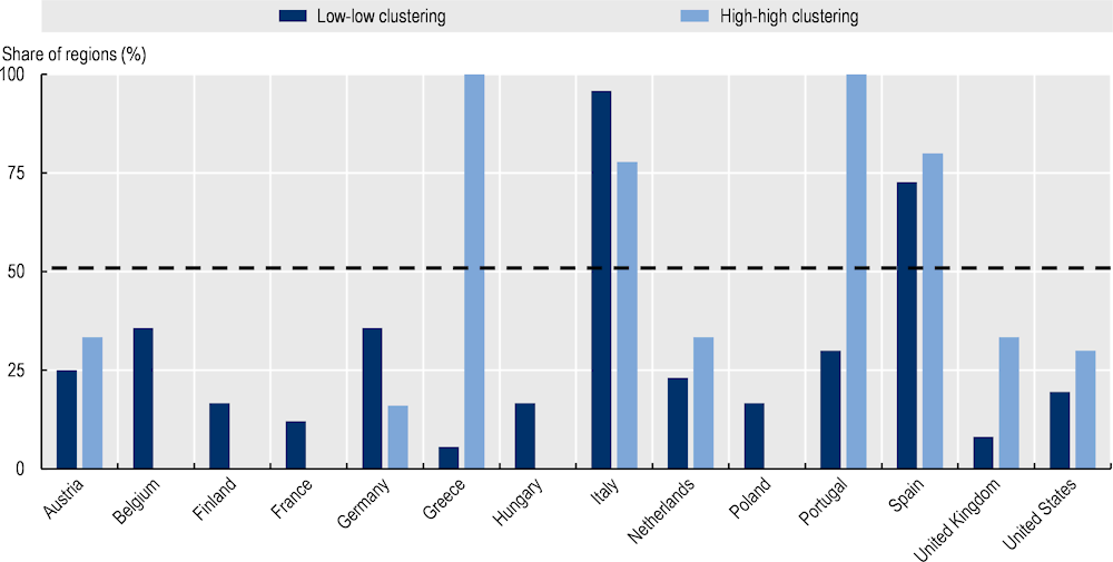
Note: The incidence of low-low spatial clustering is equal to the share of the bottom 20% of regions featuring statistically significant positive spatial clustering (i.e. spatially clustered among other low GDP per capita regions); the incidence of high-high spatial clustering is equal to the share of top 20% regions featuring statistically significant positive spatial clustering (i.e. spatially clustered among other high GDP per capita regions). Data refer to 2019. Only countries with at least 15 TL3 regions are represented.
Source: OECD (2022[33]), OECD Regional Statistics (database), https://www.oecd.org/regional/regional-statistics/.
Box 2.6. Measuring the degree of (dis)similarity among neighbouring regions
The degree of similarity of a given region with its neighbours can be measured by the Local Moran’s :
where is a socio-economic indicator for region , for instance, regional GDP per capita. The Local Moran’s can take positive, negative or zero values: positive values indicate that a given region is similar in terms of a pre-specified economic indicator to its neighbours; negative values indicate that it tends to be different from its neighbours; while a zero value means that there is no correlation with neighbours’ socio‑economic conditions. The Local Moran’s might not be sufficiently precisely estimated, in which case the data are said to rule against the existence of spatial similarity/dissimilarity among contiguous regions. If the Local Moran’s is sufficiently precisely estimated and takes on a positive value, the region is said to be clustered around regions with a similar level of income.
Figure 2.16. Measuring the degree (dis)similarity among neighbouring regions: An example based on GDP per capita in Spanish TL3 regions
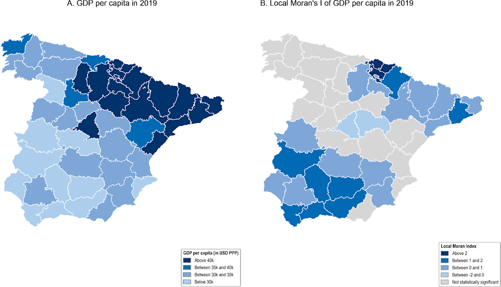
Note: The Local Moran’s is considered statistically significant when its p-values are below 20%.
Source: OECD (2022[33]), OECD Regional Statistics (database), https://www.oecd.org/regional/regional-statistics/.
Figure 2.16 provides a working example of how the measurement of spatial clustering works in practice based on the level of GDP per capita registered in Spanish TL3 regions in 2019. The left panel shows GDP per capita levels, while the right panel shows the value for the estimated Local Moran’s , whenever statistically significant. A few things merit attention. First, the Local Moran’s is not always statistically significant. Second, when a given region is surrounded by a set of regions with a level of GDP per capita very different from its own, the Local Moran’s takes on negative values (e.g. the Comunidad de Madrid or the region of Guadalajara in the central part of Spain). This is a situation opposite to the one of spatial clustering, also labelled a “checkerboard pattern”. Third, the vast majority of regions such that the Local Moran’s is sufficiently precisely estimated feature spatial clustering. Fourth, in the case of Spain, the degree of spatial clustering among regions with low GDP per capita (i.e. in the south of Spain) is higher than among regions with high GDP per capita (i.e. the northwest part of the country).
Annex 2.A. OECD regional data and methodological notes
OECD territorial definitions and administrative fragmentation
Regions are subnational units below national boundaries. OECD countries have two regional levels: large (TL2) regions and small (TL3) regions. Regional boundaries correspond to administrative divisions defined autonomously by countries using different criteria. Except for the United States, small regions are nested within large regions. However, in Estonia, Latvia and Luxembourg, TL2 borders correspond to national borders, and in Israel and New Zealand, TL2 and TL3 borders are the same. Below small regions, countries define local units such as municipalities, which are usually nested within small regional boundaries. Regional boundaries, especially those at lower scales, may be subject to changes across time as regions merge and split following demographic and political changes.
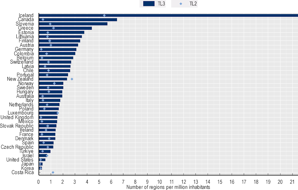
The comparison of inequality levels and rankings between territorial levels is not meaningful because the way information is scaled down varies across countries.9 The level of administrative fragmentation – that is, how national territories are split by administrative units – varies across OECD countries, especially at the TL3 level. At the TL2 level, the number of TL2 regions per 1 million inhabitants varies from 0.08 in Japan to 5.4 in Iceland. At the TL3 level, it varies from 0.33 in Korea to almost 8 regions per 1 million inhabitants in Canada (that is, 293 regions in approximately 38 million people).
Annex Figure 2.A.1. Number of TL2 and TL3 regions per million inhabitants, 2021
Source: OECD (2022[33]), OECD Regional Statistics (database), https://www.oecd.org/regional/regional-statistics/.
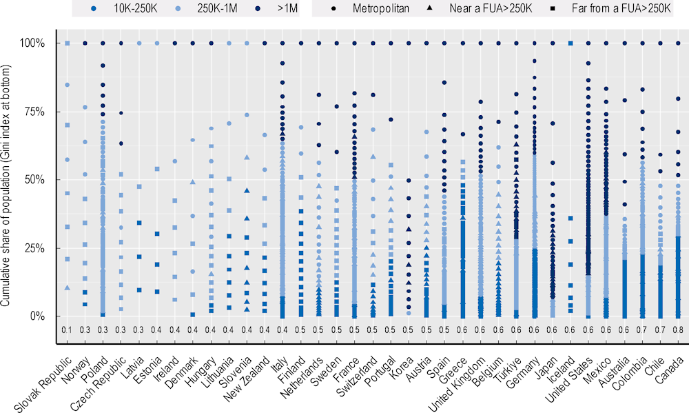
The distribution of population across regions in OECD countries is uneven. Highly urbanised countries such as the United States and sparsely populated countries such as Australia and Spain show more disparity in the distribution of population across regions. Australia has the most unequal distribution of population across small regions, as just 5 of its 51 regions account for 60% of the national population). In contrast, the populations of East European countries, Israel and the United Kingdom are more evenly distributed.
Population concentration is not always associated with large population sizes. Large and highly urbanised countries such as Japan and the United States have numerous regions with at least 1 million inhabitants and many metropolitan (large) regions (Annex Figure 2.A.2). Furthermore, countries may have similar population levels but different concentration levels. For instance, France and the United Kingdom have similar population levels but population and employment in the United Kingdom are less concentrated. The United Kingdom also has only a few small regions with over 1 million inhabitants while France has many. Though surprising when considering both countries have similar sizes, the United Kingdom has higher administrative fragmentation (see Annex Figure 2.A.1). For instance, 21 different small regions make up Greater London while only 8 make up Île-de-France. For this reason, the data in this chapter aggregate values for TL3 regions that are part of the same FUA (i.e. where 50% of the regional population lives in a FUA).
Annex Figure 2.A.2. The cumulative share of population by TL3 regions, OECD countries, 2021
Note: Excludes countries with no more than one region (Luxembourg).
Source: OECD (2022[33]), OECD Regional Statistics (database), https://www.oecd.org/regional/regional-statistics/.
The concentration of population in some countries depends on the territorial scale used. This is due to a combination of larger sparsity and the relative level of administrative fragmentation). For instance, the Gini index for the population in Denmark and Finland, 2 countries with similar population sizes, is 0.2 and 0.3 for large regions. For small regions, the Gini index is still 0.2 for Denmark (1 out of the 11 regions concentrates 15% of the population) but raises to 0.5 in Finland (1 out of the 19 regions concentrates 30% of the population) (Annex Figure 2.A.2). Higher sparsity in Finland, as well as different levels of administrative fragmentation, explain these differences. As disentangling these effects is not possible, this chapter does not make direct comparisons of inequality indicators between small and large regions.
The Access to City typology
Traditional measures of inequality such as the Theil and Gini indices do not consider the location of regions and fail to acknowledge that economic activity and people tend to cluster in space (Rey, Arribas-Bel and Wolf, 2020[62]). The OECD has developed the concept of functional urban areas – composed of urban centres and their commuting areas – to overcome these limitations. At the regional level, the OECD Access to Cities typology offers a way to overcome the issue of administrative fragmentation and lack of consideration for proximity (Fadic et al., 2019[70]).
The typology classifies small (TL3) regions into metropolitan and non-metropolitan regions according to the following criteria:
Metropolitan regions, if more than half of the population live in a FUA. Metropolitan regions are further classified into: metropolitan large, if more than half of the population live in a (large) FUA of at least 1.5 million inhabitants; and metropolitan midsize, if more than half of the population live in a (midsize) FUA of at 250 000 to 1.5 million inhabitants.
Non-metropolitan regions, if less than half of the population live in a midsize/large FUA. These regions are further classified according to their level of access to FUAs of different sizes: near a midsize/large FUA if more than half of the population live within a 60-minute drive from a midsize/large FUA (of more than 250 000 inhabitants) or if the TL3 region contains more than 80% of the area of a midsize/large FUA; near a small FUA if the region does not have access to a midsize/large FUA and at least half of its population have access to a small FUA (i.e. between 50 000 and 250 000 inhabitants) within a 60-minute drive, or contains 80% of the area of a small FUA; and remote, otherwise.
How territorial units affect the measuring of inequality
Inequality measures are sensitive to the grouping of observations in bins. For instance, measures of inter-personal inequality use income-range bins, which vary in the number of income groups available and censoring of the highest categories. The spatial counterpart of income bins are spatial units, implying that inequality indices will depend on the geographical scale of analysis. The implicit assumption, in this case, is that income in a region is equally distributed across the population in that region (Rey, Arribas-Bel and Wolf, 2020[62]).
The direction of the change in inequality when switching from a larger (TL2) to a smaller scale depends not only on the relative fragmentation at lower levels but also on the distribution of the population. For instance, consider a country with 2 TL2 regions, one with 125 people, 100 of which live in a city and another one with 42 people, 40 of which live in a city. Splitting both TL2 regions into 4 TL3 regions, 2 of them containing the 2 cities, leads to smaller inequality levels at the TL3 level, as the largest region contribution to population goes down from 75% (125/167) to 60% (100/167). Across OECD countries, switching from the TL2 to the TL3 level leads to higher, similar and lower levels of inequality in the distribution of the population (Annex Figure 2.A.3).
Annex Figure 2.A.3. Difference in Gini coefficient of population distribution between TL2 and TL3 levels, based on 2021 population values
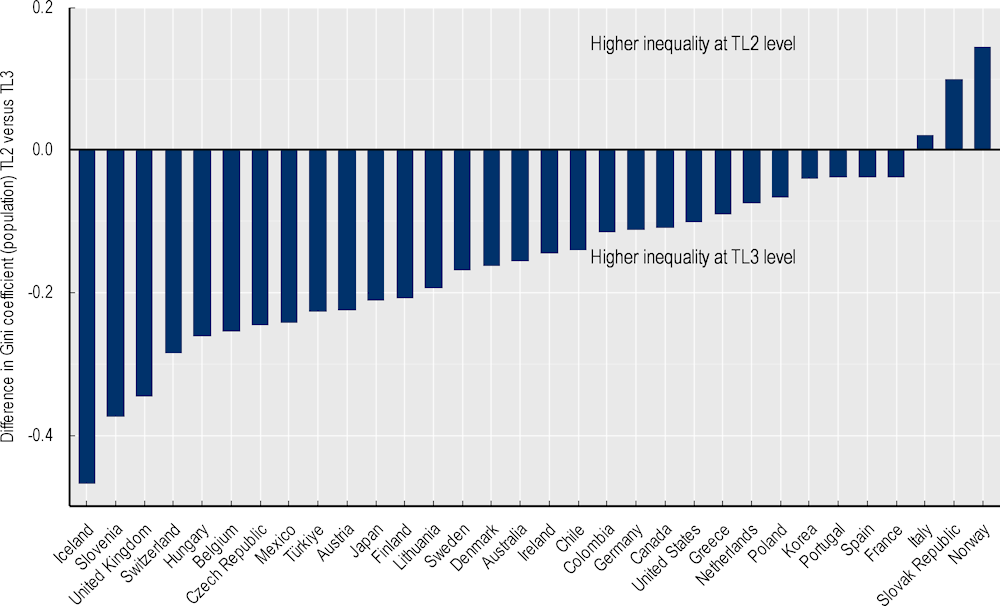
Note: Estonia, Israel, Latvia, Luxembourg and New Zealand are not included as TL2 and TL3 levels coincide. No TL3 data are available for Costa Rica.
Source: OECD (2022[33]), OECD Regional Statistics (database), https://www.oecd.org/regional/regional-statistics/.
Annex 2.B. Summary tables
Annex Table 2.B.1. Summary GDP per capita regional (TL3) inequality measures by country, 2000‑20
|
Theil index |
Top/bottom |
Top/mean |
Bottom/mean |
|||||
|---|---|---|---|---|---|---|---|---|
|
2000-09 |
2010-20 |
2000-09 |
2010-20 |
2000-09 |
2010-20 |
2000-09 |
2010-20 |
|
|
|
Mostly increasing inequality (linear) |
|||||||
|
Belgium |
0.03 |
0.03 |
2.03 |
2.03 |
1.58 |
1.56 |
0.78 |
0.77 |
|
Denmark |
0.01 |
0.02 |
1.56 |
1.68 |
1.32 |
1.39 |
0.85 |
0.82 |
|
Estonia |
0.07 |
0.08 |
2.36 |
2.48 |
1.78 |
1.83 |
0.76 |
0.74 |
|
France |
0.02 |
0.02 |
2.27 |
2.46 |
1.93 |
2.08 |
0.85 |
0.84 |
|
United Kingdom |
0.03 |
0.03 |
2.14 |
2.23 |
1.71 |
1.78 |
0.80 |
0.80 |
|
Sweden |
0.01 |
0.01 |
1.73 |
1.79 |
1.58 |
1.60 |
0.91 |
0.90 |
|
|
Mostly increasing inequality (non-linear) |
|||||||
|
Czech Republic |
0.02 |
0.02 |
2.05 |
2.10 |
1.77 |
1.79 |
0.86 |
0.85 |
|
Hungary |
0.04 |
0.05 |
2.72 |
2.66 |
1.99 |
1.96 |
0.73 |
0.74 |
|
Italy |
0.03 |
0.04 |
2.32 |
2.43 |
1.56 |
1.62 |
0.67 |
0.67 |
|
Japan |
0.01 |
0.01 |
1.53 |
1.47 |
1.36 |
1.30 |
0.89 |
0.89 |
|
Lithuania |
0.04 |
0.05 |
2.25 |
2.32 |
1.71 |
1.77 |
0.76 |
0.76 |
|
Poland |
0.04 |
0.05 |
2.50 |
2.72 |
1.89 |
1.98 |
0.76 |
0.73 |
|
Slovak Republic |
0.11 |
0.11 |
2.90 |
3.01 |
1.75 |
1.83 |
0.61 |
0.61 |
|
Slovenia |
0.02 |
0.03 |
1.98 |
1.97 |
1.62 |
1.63 |
0.82 |
0.83 |
|
United States |
0.02 |
0.03 |
1.76 |
1.90 |
1.50 |
1.56 |
0.85 |
0.82 |
|
|
Mostly decreasing inequality (linear) |
|||||||
|
Finland |
0.02 |
0.01 |
1.83 |
1.67 |
1.53 |
1.47 |
0.84 |
0.88 |
|
Greece |
0.03 |
0.03 |
1.99 |
2.04 |
1.56 |
1.65 |
0.79 |
0.81 |
|
Latvia |
0.07 |
0.06 |
2.64 |
2.44 |
1.74 |
1.72 |
0.66 |
0.71 |
|
Norway |
0.04 |
0.03 |
1.94 |
1.90 |
1.59 |
1.54 |
0.82 |
0.81 |
|
Portugal |
0.03 |
0.02 |
2.24 |
1.88 |
1.70 |
1.54 |
0.76 |
0.82 |
|
Türkiye |
0.07 |
0.06 |
3.68 |
3.36 |
2.26 |
2.16 |
0.61 |
0.64 |
|
|
Mostly decreasing inequality (non-linear) |
|||||||
|
Austria |
0.02 |
0.02 |
1.74 |
1.57 |
1.36 |
1.26 |
0.78 |
0.80 |
|
Germany |
0.04 |
0.04 |
2.25 |
2.05 |
1.67 |
1.57 |
0.74 |
0.77 |
|
Spain |
0.02 |
0.02 |
1.79 |
1.84 |
1.41 |
1.45 |
0.79 |
0.79 |
|
Korea |
0.06 |
0.05 |
1.81 |
1.85 |
1.29 |
1.30 |
0.71 |
0.70 |
|
Netherlands |
0.02 |
0.02 |
1.72 |
1.68 |
1.43 |
1.43 |
0.83 |
0.85 |
|
New Zealand |
0.02 |
0.02 |
1.58 |
1.52 |
1.29 |
1.24 |
0.82 |
0.82 |
Note: Countries with GDP per capita above OECD levels in 2000 and 2020 are listed in bold.
Top/bottom calculated as population equivalent (top/bottom regions with at least 20% of the population). The interpretation of top/bottom 20% GDP per capita is that 20% of the population in the country holds 20% of the value.
Source: OECD (2022[33]), OECD Regional Statistics (database), https://www.oecd.org/regional/regional-statistics/.
Annex Table 2.B.2. Summary table of the share of between-group inequality across TL3 region types, 2000-20
|
|
Large metropolitan vs. the rest |
Metropolitan vs. the rest |
Far from a FUA>250K vs. the rest |
|||
|---|---|---|---|---|---|---|
|
2000-09 |
2010-20 |
2000-09 |
2010-20 |
2000-09 |
2010-20 |
|
|
|
Large metropolitan/Top vs. the rest |
|||||
|
Czech Republic |
3.64 |
2.75 |
0.80 |
0.80 |
0.69 |
0.75 |
|
Denmark |
2.01 |
1.85 |
1.26 |
1.14 |
1.10 |
1.00 |
|
France |
1.04 |
1.04 |
0.87 |
0.90 |
0.73 |
0.74 |
|
Hungary |
1.94 |
1.45 |
1.31 |
1.21 |
1.10 |
1.06 |
|
Korea |
1.67 |
1.49 |
1.20 |
1.14 |
||
|
Poland |
1.63 |
1.25 |
1.14 |
1.08 |
0.83 |
0.86 |
|
Portugal |
1.24 |
1.01 |
0.94 |
0.92 |
0.96 |
0.94 |
|
Sweden |
3.06 |
2.15 |
1.01 |
1.04 |
0.87 |
0.97 |
|
Türkiye |
1.46 |
1.19 |
1.04 |
0.91 |
1.08 |
1.01 |
|
United Kingdom |
1.79 |
1.52 |
1.27 |
1.13 |
0.55 |
0.52 |
|
United States |
2.18 |
1.71 |
1.20 |
0.99 |
0.95 |
0.86 |
|
|
Metropolitan/Top vs. the rest |
|||||
|
Belgium |
0.59 |
0.40 |
0.99 |
0.88 |
0.31 |
0.33 |
|
Estonia |
1.90 |
1.71 |
1.64 |
1.60 |
||
|
Finland |
1.19 |
1.11 |
1.03 |
1.03 |
||
|
Latvia |
1.60 |
1.59 |
1.39 |
1.48 |
||
|
Lithuania |
1.24 |
1.21 |
1.07 |
1.13 |
||
|
Norway |
0.94 |
0.93 |
0.82 |
0.87 |
||
|
Slovak Republic |
1.26 |
1.20 |
0.80 |
0.79 |
||
|
Spain |
1.18 |
1.11 |
1.41 |
1.29 |
1.20 |
1.16 |
|
Netherlands |
1.33 |
1.06 |
1.19 |
1.07 |
||
|
|
Metropolitan vs. the rest |
|||||
|
Germany |
0.99 |
0.93 |
1.22 |
1.11 |
0.63 |
0.55 |
|
Japan |
1.54 |
1.10 |
1.21 |
1.18 |
0.38 |
0.34 |
|
New Zealand |
1.46 |
1.13 |
1.26 |
1.05 |
||
|
Slovenia |
1.21 |
0.96 |
0.99 |
0.85 |
||
|
|
Far from a FUA>250K vs. the rest |
|||||
|
Austria |
0.49 |
0.43 |
0.77 |
0.62 |
1.37 |
1.27 |
|
Greece |
1.11 |
0.61 |
0.79 |
0.58 |
1.04 |
1.11 |
|
Italy |
0.65 |
0.63 |
0.88 |
0.81 |
1.15 |
1.12 |
Note: Values relative to the OECD mean. Countries with increasing inequalities are listed in bold. Regions with null values do not have regions of the corresponding type.
Source: OECD (2022[33]), OECD Regional Statistics (database), https://www.oecd.org/regional/regional-statistics/.
References
[22] Ahlfeldt, G. and E. Pietrostefani (2019), “The economic effects of density: A synthesis”, Journal of Urban Economics, Vol. 111, pp. 93-107, https://doi.org/10.1016/j.jue.2019.04.006.
[18] Autor, D., D. Dorn and G. Hanson (2013), “The geography of trade and technology shocks in the United States”, American Economic Review, Vol. 103/3, pp. 220-225, https://doi.org/10.1257/aer.103.3.220.
[71] Balestra, C. and R. Tonkin (2018), “Inequalities in household wealth across OECD countries: Evidence from the OECD Wealth Distribution Database”, OECD Statistics Working Papers, No. 2018/01, OECD Publishing, Paris, https://doi.org/10.1787/7e1bf673-en.
[66] Boulant, J., M. Brezzi and P. Veneri (2016), “Income Levels And Inequality in Metropolitan Areas: A Comparative Approach in OECD Countries”, OECD Regional Development Working Papers, No. 2016/6, OECD Publishing, Paris, https://doi.org/10.1787/5jlwj02zz4mr-en.
[4] Combes, P. et al. (2011), “The rise and fall of spatial inequalities in France: A long-run perspective”, Explorations in Economic History, Vol. 48/2, pp. 243-271, https://doi.org/10.1016/j.eeh.2010.12.004.
[17] Diemer, A. et al. (2022), “The regional development trap in Europe”, Economic Geography, pp. 1-23, https://doi.org/10.1080/00130095.2022.2080655.
[21] Dijkstra, L., E. Garcilazo and P. McCann (2013), “The economic performance of European cities and city regions: Myths and realities”, European Planning Studies, Vol. 21/3, pp. 334-354, https://doi.org/10.1080/09654313.2012.716245.
[12] Dijkstra, L., H. Poelman and A. Rodríguez-Pose (2019), “The geography of EU discontent”, Regional Studies, Vol. 54/6, pp. 737-753, https://doi.org/10.1080/00343404.2019.1654603.
[15] EC (2022), Cohesion in Europe towards 2050: Eighth Report on Economic, Social and Territorial Cohesion, European Commission.
[64] Elbers, C. et al. (2008), Re-Interpreting between-group inequality, pp. 231-245, https://link.springer.com/article/10.1007/s10888-007-9064-x.
[39] Eurostat (2022), European Union Labour Force Survey, https://ec.europa.eu/eurostat/web/microdata/european-union-labour-force-survey.
[70] Fadic, M. et al. (2019), “Classifying small (TL3) regions based on metropolitan population, low density and remoteness”, OECD Regional Development Working Papers, No. 2019/06, OECD Publishing, Paris, https://doi.org/10.1787/b902cc00-en.
[60] Faggian, A. and A. Ascani (2021), “Productivity and resilience. A post-COVID-19 perspective”, OECD-EC high-level expert workshop series Productivity Policy for Places, OECD, Paris, https://www.oecd.org/regional/W5-S1-Alessandra-Faggian-Andrea-Ascani.pdf (accessed on 31 January 2022).
[58] Garcilazo, E., A. Moreno-Monroy and J. Oliveira Martins (2021), “Regional inequalities and contributions to aggregate growth in the 2000s: An EU vs US comparison based on functional regions”, Oxford Review of Economic Policy, Vol. 37/1, pp. 70-96, https://doi.org/10.1093/oxrep/graa064.
[3] Glaeser, E. and J. Gottlieb (2009), “The wealth of cities: Agglomeration economies and spatial equilibrium in the United States”, Journal of Economic Literature, Vol. 47/4, pp. 983-1028, https://doi.org/10.1257/jel.47.4.983.
[61] Gluschenko, K. (2017), “Measuring regional inequality: To weight or not to weight?”, Spatial Economic Analysis, Vol. 13/1, pp. 36-59, https://doi.org/10.1080/17421772.2017.1343491.
[10] Hanushek, E. and L. Woessmann (2020), “The economic impacts of learning losses”, OECD, Paris, https://www.oecd.org/education/The-economic-impacts-of-coronavirus-covid-19-learning-losses.pdf.
[1] Hirschman, A. and M. Rothschild (1973), “The changing tolerance for income inequality in the course of economic development”, The Quarterly Journal of Economics, Vol. 87/4, pp. 544-566, https://www.jstor.org/stable/1882024#metadata_info_tab_contents.
[49] Hsia, R. et al. (2012), “Is emergency department closure resulting in increased distance to the nearest emergency department associated with increased inpatient mortality?”, Annals of Emergency Medicine, Vol. 60/6, pp. 707-715.e4, https://doi.org/10.1016/j.annemergmed.2012.08.025.
[69] Iammarino, S., A. Rodríguez-Pose and M. Storper (2019), “Regional inequality in Europe: Evidence, theory and policy implications”, Journal of Economic Geography, Vol. 19/2, pp. 273-298, https://academic.oup.com/joeg/article/19/2/273/4989323.
[46] Institute for Fiscal Studies (2021), London Calling? Higher Education, Geographical Mobility and Early-career Earnings, https://assets.publishing.service.gov.uk/government/uploads/system/uploads/attachment_data/file/1022365/London_calling_final_for_dfe_with_accessibility.pdf.
[47] JRC (2022), New Perspectives on Territorial Disparities: From Lonely Places to Places of Opportunities, Joint Research Centre, European Commission, https://op.europa.eu/en/publication-detail/-/publication/8fcaf458-f1da-11ec-a534-01aa75ed71a1/language-en.
[8] Kemeny, T. and M. Storper (2020), “Superstar cities and left-behind places: Disruptive innovation, labor demand, and interregional inequality”, International Inequalities Institute, London School of Economics and Political Science, http://eprints.lse.ac.uk/103312/1/Kemeny_superstar_cities_left_behind_place_wp41.pdf.
[63] Königs, S. et al. (forthcoming), “The geography of income inequalities in OECD countries: Evidence from national register data”, OECD Publishing, Paris.
[2] Kuznets, S. (1955), “Economic growth and income inequality”, American Economic Review, Vol. 45, pp. 1-28.
[9] Manduca, R. (2019), “The contribution of national income inequality to regional economic divergence”, Social Forces, Vol. 98/2, pp. 622-648, https://doi.org/10.1093/sf/soz013.
[41] Mapbox (2022), Navigation, https://docs.mapbox.com/api/navigation/.
[65] McCann, P. (2022), “The differential economic geography of regional and urban growth and prosperity in industrialised countries”, GOLD VI Working Paper Series, No. 13, https://gold.uclg.org/sites/default/files/13_the_differential_economic_geography_of_regional_and_urban_growth_and_prosperity_in_industrialised_countries_by_philip_mccann.pdf.
[6] Moretti, E. (2012), The New Geography Of Jobs, Houghton Mifflin Harcourt.
[19] Navaretti, G. and B. Markovic (2021), “Place-based policies and the foundations of productivity in the private sector: What are we building on?”, OECD-EC high-level expert workshop Productivity Policy for Places, OECD, Paris.
[29] OECD (2022), Adapting Regional Policy in Korea: Preparing Regions for Demographic Change, OECD Rural Studies, OECD Publishing, Paris, https://doi.org/10.1787/6108b2a1-en.
[14] OECD (2022), Addressing territorial disparities in future infrastructure needs in the wake of the COVID-19 crisis: A G20 perspective, OECD Publishing, Paris, https://doi.org/10.1787/e246f50f-en.
[40] OECD (2022), “ADHEP database”, Unpublished, OECD, Paris.
[43] OECD (2022), Delivering Quality Services to All in Alentejo: Preparing Regions for Demographic Change, OECD Rural Studies, OECD Publishing, Paris, https://doi.org/10.1787/63ffb4d7-en.
[42] OECD (2022), Education at a Glance 2022: OECD Indicators, OECD Publishing, Paris, https://doi.org/10.1787/3197152b-en.
[37] OECD (2022), International Migration Outlook 2022, OECD Publishing, Paris, https://doi.org/10.1787/30fe16d2-en.
[59] OECD (2022), “Making the most of public investment to address regional inequalities, megatrends and future shocks”, OECD Regional Development Papers, No. 29, OECD Publishing, Paris, https://doi.org/10.1787/8a1fb523-en.
[33] OECD (2022), OECD Regional Statistics (database), OECD, Paris, https://www.oecd.org/regional/regional-statistics/.
[36] OECD (2022), OECD Regions and Cities at a Glance 2022, OECD Publishing, Paris, https://doi.org/10.1787/14108660-en.
[44] OECD (2022), Resourcing Higher Education in Portugal, Higher Education, OECD Publishing, Paris, https://doi.org/10.1787/a91a175e-en.
[38] OECD (2022), The Contribution of Migration to Regional Development, OECD Regional Development Studies, OECD Publishing, Paris, https://doi.org/10.1787/57046df4-en.
[45] OECD (2022), Unlocking Rural Innovation, OECD Rural Studies, OECD Publishing, Paris, https://doi.org/10.1787/9044a961-en.
[51] OECD (2021), Bridging digital divides in G20 countries, OECD Publishing, Paris, https://doi.org/10.1787/35c1d850-en.
[11] OECD (2021), Delivering Quality Education and Health Care to All: Preparing Regions for Demographic Change, OECD Rural Studies, OECD Publishing, Paris, https://doi.org/10.1787/83025c02-en.
[20] OECD (2021), “Regions and globalisation: An original approach to regional internationalisation and its application to the case of France”, OECD Regional Development Papers, No. 20, OECD Publishing, Paris, https://doi.org/10.1787/75dae685-en.
[13] OECD (2020), “A systemic resilience approach to dealing with Covid-19 and future shocks”, OECD Policy Responses to Coronavirus (COVID-19), OECD, Paris, https://www.oecd.org/coronavirus/policy-responses/a-systemic-resilience-approach-to-dealing-with-covid-19-and-future-shocks-36a5bdfb/.
[52] OECD (2020), OECD Regions and Cities at a Glance 2020, OECD Publishing, Paris, https://doi.org/10.1787/959d5ba0-en.
[50] OECD (2020), “Policy implications of Coronavirus crisis for rural development”, OECD Policy Responses to Coronavirus (COVID-19), OECD, Paris, https://www.oecd.org/coronavirus/policy-responses/policy-implications-of-coronavirus-crisis-for-rural-development-6b9d189a/.
[16] OECD (2020), Rural Well-being: Geography of Opportunities, OECD Rural Studies, OECD Publishing, Paris, https://doi.org/10.1787/d25cef80-en.
[28] OECD (2019), Declaration on Policies for Building Better Futures for Regions, Cities and Rural Areas, OECD, Paris, https://www.oecd.org/regional/ministerial/RDPC-Ministerial-Declaration-EN.pdf.
[56] OECD (2019), Promoting Healthy Ageing: Background Report for the 2019 Japanese G20 Presidency, OECD, Paris, https://www.oecd.org/g20/topics/global-health/G20-report-promoting-healthy-ageing.pdf (accessed on May 2022).
[30] OECD (2018), OECD Rural Policy Reviews: Poland 2018, OECD Rural Policy Reviews, OECD Publishing, Paris, https://doi.org/10.1787/9789264289925-en.
[27] OECD (2014), How’s Life in Your Region?: Measuring Regional and Local Well-being for Policy Making, OECD Regional Development Studies, OECD Publishing, Paris, https://doi.org/10.1787/9789264217416-en.
[26] OECD (2012), Promoting Growth in All Regions, OECD Regional Development Studies, OECD Publishing, Paris, https://doi.org/10.1787/9789264174634-en.
[25] OECD (2011), OECD Regional Outlook 2011: Building Resilient Regions for Stronger Economies, OECD Publishing, Paris, https://doi.org/10.1787/9789264120983-en.
[24] OECD (2009), How Regions Grow: Trends and Analysis, OECD Regional Development Studies, OECD Publishing, Paris, https://doi.org/10.1787/9789264039469-en.
[48] OECD/EC (2020), Cities in the World: A New Perspective on Urbanisation, OECD Urban Studies, OECD Publishing, Paris, https://doi.org/10.1787/d0efcbda-en.
[32] OECD et al. (2021), Applying the Degree of Urbanisation: A Methodological Manual to Define Cities, Towns and Rural Areas for International Comparisons, OECD Regional Development Studies, OECD Publishing, Paris/European Union, Brussels, https://doi.org/10.1787/4bc1c502-en.
[68] Parry, J. (2022), “sfdep: Spatial dependence for simple features”, https://github.com/josiahparry/sfdep.
[5] Puga, D. (1999), “The rise and fall of regional inequalities”, European Economic Review, Vol. 43/2, pp. 303-334, https://doi.org/10.1016/s0014-2921(98)00061-0.
[62] Rey, S., D. Arribas-Bel and L. Wolf (2020), “Spatial inequality dynamics”, in Geographic Data Science with Python, https://geographicdata.science/book/notebooks/09_spatial_inequality.html (accessed on June 2022).
[67] Rey, S. and R. Smith (2012), “A spatial decomposition of the Gini coefficient”, Letters in Spatial and Resource Sciences, Vol. 6/2, pp. 55-70, https://doi.org/10.1007/s12076-012-0086-z.
[57] Rice, P. and A. Venables (2020), “The persistent consequences of adverse shocks: How the 1970s shaped UK regional inequality”, CEPR Discussion Paper, No. DP15261.
[72] Rosés, J. and N. Wolf (2018), “Regional economic development in Europe, 1900–2010: A description of the patterns”, CEPR Discussion Papers, No. 12749, https://cepr.org/publications/dp12749.
[55] Rouzet, D. et al. (2019), “Fiscal challenges and inclusive growth in ageing societies”, OECD Economic Policy Papers, No. 27, OECD Publishing, Paris, https://doi.org/10.1787/c553d8d2-en (accessed on 18 January 2022).
[34] Schiavina, M. et al. (2023), GHSL Data Package 2023, Publications Office of the European Union, https://doi.org/10.2760/098587.
[35] Souder, A. et al. (2021), “Going granular - A new database on migration in municipalities across the OECD”, OECD Regional Development Working Papers, OECD, Paris.
[7] Südekum, J. (2021), “Place-based policies - How to do them and why”, DICE Discussion Paper, No. 367, https://www.econstor.eu/bitstream/10419/237051/1/1767077793.pdf.
[73] Trapeznikova, I. (2019), “Measuring income inequality”, IZA World of Labor, https://doi.org/10.15185/izawol.462.
[31] UK Government (2022), “Levelling up the United Kingdom”, https://www.gov.uk/government/publications/levelling-up-the-united-kingdom.
[23] Venables, A. (2018), “Globalization and urban polarization”, Review of International Economics, Vol. 26/5, pp. 981-996, https://onlinelibrary.wiley.com/doi/full/10.1111/roie.12366.
[54] Vollset, S. et al. (2020), “Fertility, mortality, migration, and population scenarios for 195 countries and territories from 2017 to 2100: A forecasting analysis for the Global Burden of Disease Study”, The Lancet, Vol. 396/10258, pp. 1285-1306, https://doi.org/10.1016/s0140-6736(20)30677-2.
[53] Weiss, D. et al. (2020), “Global maps of travel time to healthcare facilities”, Nature Medicine, Vol. 26/12, pp. 1835-1838, https://doi.org/10.1038/s41591-020-1059-1.
Notes
← 1. These is the ratio between the 20% richest and 20% poorest population’s disposable income.
← 2. The OECD Programme for International Student Assessment (PISA) is an international assessment that measures 15-year-old students’ reading, mathematics and science literacy every 3 years.
← 3. The rest of the document uses the terms GDP per capita and income per capita interchangeably.
← 4. Additionally: GDP and population may not be recorded at the same place (place of residency versus place of work); national deflators do not consider higher living costs in cities and GDP value in some services such as financial services and real state may be distorted by where transactions are recorded.
← 5. Values above 1 of this ratio indicate the presence of regions with very high or very low values relative to the mean. This indicator has been used to analyse inter-personal inequalities in OECD countries (Balestra and Tonkin, 2018[71]).
← 6. The absolute value differs because each measure uses all the countries with available data (26 OECD at the TL3 and 29 OECD countries at the TL2 level. The trends are identical when using the same group of 23 OECD countries at both levels.
← 7. The absolute gap in income per head between top and bottom regions can increase even when polarisation measured with the ratio of GDP per capita in top versus bottom regions decreases. Given higher GDP per capita income in top than in bottom regions (e.g. EUR 50 000 vs EUR 10 000), when top and bottom regions grow at exactly the same rate (e.g. 10%) the absolute gap between top and bottom increases (by EUR 400, i.e. EUR 50 500 minus EUR 10 100) and the relative gap stays the same (5 in both cases).
← 8. The geography of spatial clustering presented here tends to diverge from that described in Rosés and Wolf (2018[72]), who report the emergence during the twentieth century of so-called “islands of prosperity” in Europe, i.e. clusters of increasingly rich regions located typically around the largest European metropolitan areas. The main reason behind this divergence has to do with the different geographical units employed in the analysis, TL2 regions in Rosés and Wolf (2018[72]) and TL3 regions (bundling together those belonging to the same metropolitan regions) in the present analysis.
← 9. The technical reason is that no conclusive ranking between distributions can be drawn when Lorenz curves cross (Trapeznikova, 2019[73]).