Getting to Services in Towns and Villages

3. Services and transport to towns and villages

Abstract

This chapter investigates the link between service availability and the quality of transportation to settlements, whether by car or public transport. It introduces several measures of how many people can reach a town or village from the surrounding area, considering driving times or public transport trips with multiple possible transfers. The chapter examines how the number of services within a settlement relates to the number of people living inside and those living in the surrounding area who can access the settlement within a reasonable travel time. In addition, the analysis looks at several extensions: different dynamics for towns and villages, the number of services in the surrounding areas and the relative impact of being a regional centre or having one or more larger settlements nearby.

Introduction

This chapter focuses on the role of transport in connecting people to services. The topic has been widely studied in cities (Deboosere and El-Geneidy, 2018[1]; ITF, 2019[2]; Pereira et al., 2019[3]; OECD, 2020[4]) but significantly less in rural areas or smaller settlements like towns and villages. In the rural context, more central settlements, with more transport links, may serve as service hubs to wider areas. However, faster transport to and from smaller settlements as a targeted approach can yield unintended consequences, such as reducing their local service provision by increasing the accessibility of larger settlements. OECD analysis supports taking an integrated approach, whereby infrastructure improvements can have a positive impact when other factors are also present in a region, e.g. strong human capital, robust employment rates and good innovation rates (OECD, 2012[5]).

Given their declining populations, understanding the relationship between reachability, transport links and service provision in rural areas is pivotal. Many OECD regions need to plan for this demographic reality and adjust service provision for population change. This chapter uses comprehensive data on points of interest (POIs) and driving and public transport travel times to investigate whether transport infrastructure that connects the surrounding population to settlements affects their service provision.

The relationship between service provision and transport to settlements depends not only on transport networks and connections but also on the spatial distribution of the population. This chapter analyses a smaller sample of five OECD countries and one self-contained region – Estonia, Luxembourg, the Netherlands, Sweden, Switzerland and the island of Sardinia, Italy – to examine whether settlements with more effective public transport networks or faster car connectivity have more services. This chapter first describes the population, service and transit data needed to compute relevant accessibility measures. Next, it uses such measures to evaluate how the number of services inside a settlement relates to the population both inside and outside. Finally, it explores interactions between transport modes, settlement types and reachability measures to provide additional insights.

Measuring access to services by car and public transport

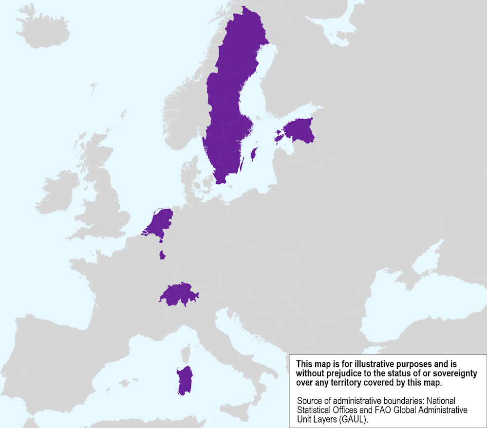
To study the relationships between transport and service provision, this chapter uses three types of data: i) population grids; ii) locations of services and travel times by public transport; and iii) private vehicle driving.1 Public transport data are particularly difficult to obtain with full coverage: thus, this chapter includes data for five countries and one region for which complete multi-modal network data can be verified (Figure 3.1). These places also have comprehensive and comparable data on population, services and car transport.

Figure 3.1. Map of countries and region included in the analysis

Population

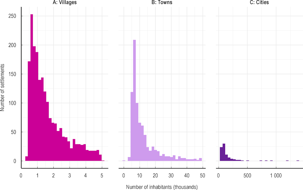
Accessible population is defined as the population that can access the settlement by car or public transport within a specified time threshold. As described in Chapter 1, one square kilometre (km²) gridded population data for Europe are available from the European GEOSTAT Census Population grid (Annex Table 1.A.3). There are more than 800 towns and 2 000 villages in these 5 countries and 1 region (Annex Table 3.A.2). Like the full dataset, the selected countries/regions have an average village size of around 1 000 inhabitants and an average town size of 8 500 inhabitants (Annex Table 3.A.3).

Figure 3.2. Population distribution for villages, towns and cities in selected countries and regions

Source: Based on data from selected countries and regions.

Statlink

Points of interest

In addition to the five services from the previous chapter (banks, higher education institutions (HEIs), hospitals, pharmacies and schools), this chapter considers cinemas, food stores and restaurants.2 As in Chapter 2, common services include banks, food stores, pharmacies, restaurants and schools – present in more than half of towns – while uncommon services include cinemas, HEIs and hospitals. Service data are available for the selected countries and region (Estonia, Luxembourg, the Netherlands, Sweden, Switzerland and Sardinia, Italy).

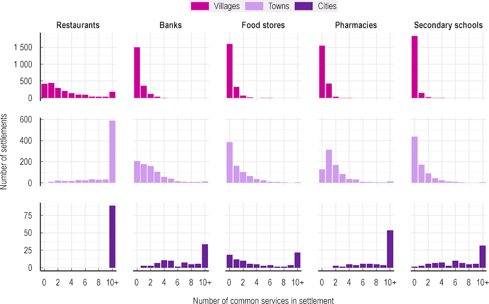
Villages and towns are more similar to each other in terms of service prevalence than cities. Figure 3.3 shows the number of common services by settlement type, with the leftmost bar in each plot indicating the number of settlements without a given service. Despite their small population sizes and limited customer demand, most villages in the sample have at least one restaurant. However, most villages have no pharmacies, banks, food stores or secondary schools, considering each service type separately (aggregates across services are tabulated below). Most towns have multiple restaurants and at least one pharmacy or bank, but 47% do not have a food store, and 54% do not have a secondary school. Many cities have more than ten of each type of common service.

Figure 3.3. Number of common services in each settlement, selected countries and regions

Source: Based on data from selected countries and regions.

Statlink

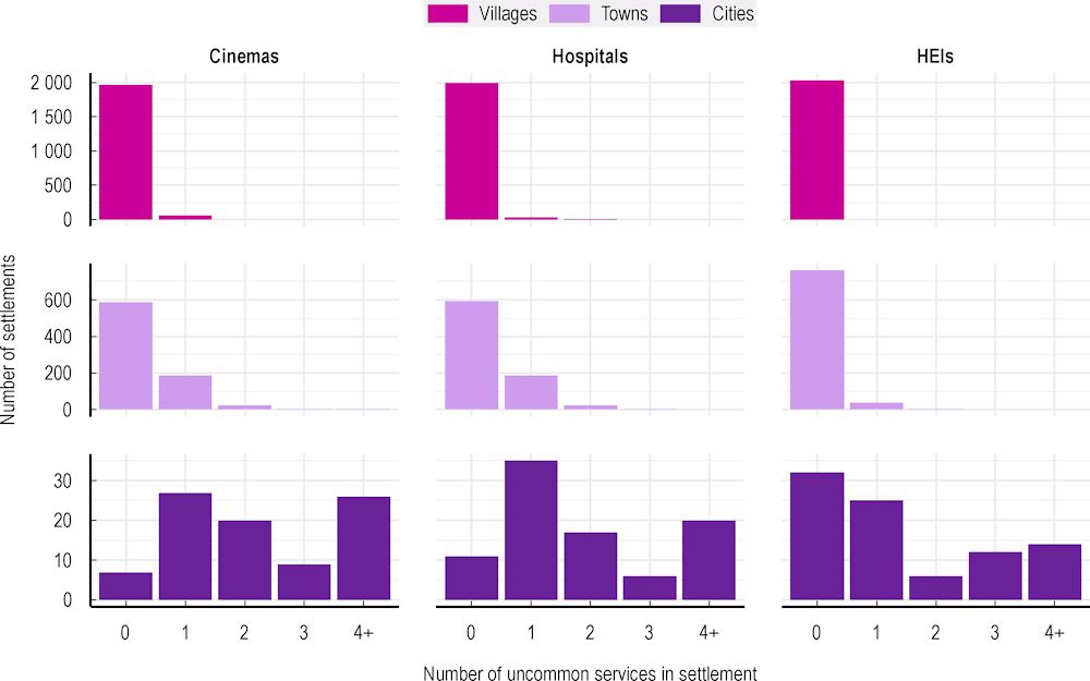
Uncommon services such as cinemas and hospitals are rare in towns and especially villages (Figure 3.4). Most towns and villages across all countries do not have any HEIs such as universities. Even cities have small numbers of uncommon services, or zero in some cases.

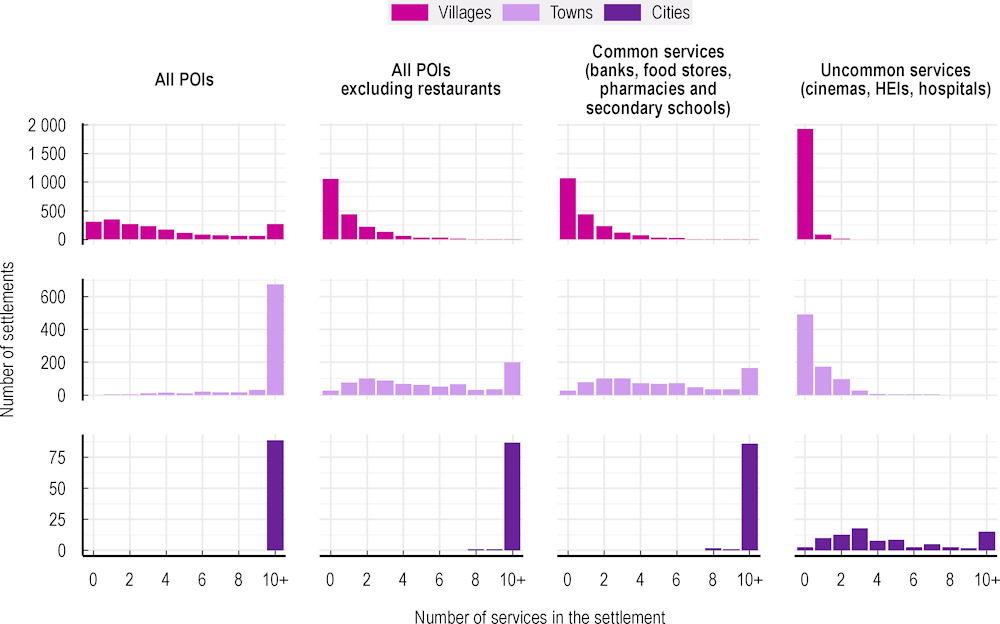
The following analysis groups the total number of POIs in four different ways: i) all services; ii) all but restaurants; iii) only common services (banks, food stores, pharmacies and secondary schools); and iv) uncommon services (only cinemas, HEIs and hospitals). The histograms in Figure 3.5 show that the distribution of total POIs in villages is relatively uniform when restaurants are included but restaurants dominate the count of service locations. In contrast, many smaller settlements do not have cinemas, HEIs or hospitals. These uncommon facilities tend to operate on a larger scale, serving a broader population across multiple settlements. Since towns and villages often have none – or at most one – of these uncommon services, they are better modelled as binary variables instead of count variables.

Figure 3.4. Number of uncommon services in each settlement, selected countries and regions

Source: Based on data from selected countries and regions.

Statlink

Figure 3.5. Number of services tabulated as POIs, selected countries and regions

Source: Based on data from selected countries and regions.

Statlink

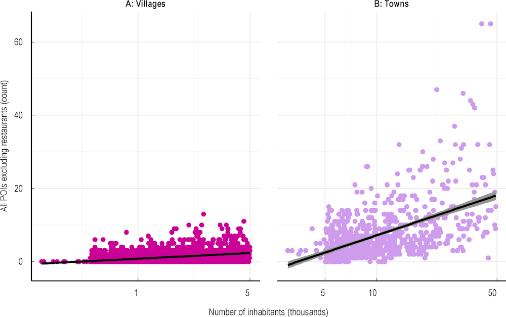
As in Chapter 2, the number of services in settlements generally increases with settlement population (Figure 3.6). This positive relationship between services and settlement population is stronger for towns than villages. The rest of the chapter builds an empirical model to assess the relationship between services inside a settlement and the size of the population that can access the settlement from outside, where the latter is informed by actual travel connections from the settlement’s surroundings.

Figure 3.6. Relationship between population and POIs excluding restaurants, towns and villages

Source: Based on data from selected countries and regions.

Statlink

Analysing accessibility to settlements

Chapter 2 considers accessibility to services within settlements. Instead, this chapter considers accessibility to services in each settlement for people travelling from outside that settlement. It examines how easily people from outside can reach the settlement by car or public transport (hereafter referred to as “PTr”) within a specific time limit, in this case 45 minutes.

Travel time calculations

The analysis compares a multi-modal PTr trip to a single car journey from a person’s place of residence to the settlement. For car accessibility, the analysis tabulates the population living within a 45-minute driving time from the surroundings of a settlement to its borders. It does not consider accessibility to the specific service location within the settlement or account for parking availability (or lack thereof) at destination.

Public transport tabulations indicate whether inhabitants living outside a settlement can get to it using common transport modes such as buses, trains and ferries. All PTr rides are calculated during morning rush hour (7.30-9.30 am), starting at any scheduled departure time and travelling up to 30 minutes within the transit network. All modes of PTr to settlements typically run at high frequency during these peak morning hours. The number of changes for a viable itinerary is capped at 4 but there is no limit on transfer distance or waiting time as long as the total ride takes less than 30 minutes. The intuition for this time threshold is that, while shorter times might limit travel to just 1 transit mode, a PTr ride of up to 30 minutes is similar to average commuting times and makes multi-modal transport possible for the wider population living nearby.

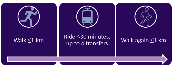
Population is assumed to be reachable if at least one viable PTr itinerary to the settlement is available. An additional buffer distance of 1 km around each transit stop ensures that the PTr measure captures the entire reachable population. Thus, the entire PTr trip is estimated to correspond to a maximum of 45 minutes: 30 minutes of actual riding in buses, trains and/or ferries and 15 minutes (total) of walking to and from the transit stops (Figure 3.7).3

Figure 3.7. Illustration of public transport accessibility measurement

The public transport calculations rely on local transport networks’ General Transit Feed Specification (GTFS) and the VelociRAPTOR algorithm developed by the European Commission’s Joint Research Centre (Tomasi C., forthcoming[6]). The minimum time from each origin grid cell to each destination settlement is assumed to be the time it takes a traveller to reach any grid cell within the settlement. In some cases, this destination grid cell may be the closest one to the origin, while in other cases, it may be the grid cell corresponding to a central travel hub (e.g. a train station inside the settlement) or another stop that is well-connected to the origin. See Annex Table 3.B.1 for more details on GTFS and the VelociRAPTOR routing algorithm and (Giordano A., forthcoming[7]) for an application.

Box 3.1 describes Canada’s Spatial Access Measures that quantify people’s access to services and amenities along Canada’s rural-urban continuum via different modes of available transport.

Box 3.1. Canada’s proximity measures

Canada’s Spatial Access Measures are the result of a collaboration between Statistics Canada and Infrastructure Canada. They measure access to services and amenities using active (walking and biking) and public (peak and non-peak) modes of transportation. The services and amenities include education (primary, secondary, post-secondary), healthcare facilities, grocery stores, cultural and arts facilities, sports and recreational facilities and places of employment. All measures are provided at the dissemination block level, which corresponds to a city block in urban areas or an area bounded by roads or other natural features in rural areas.

The Spatial Access Measures show, for example, that nearly half of Canadians live within 1 km walking distance from a grocery store. In larger metropolitan areas, 55% of people live in proximity to a grocery store compared to only 30% of those in smaller metropolitan areas and 16% in rural areas. In the rural and small town (RST) context, Canada’s ProximityRST database considers the driving distances that residents of rural communities typically encounter when accessing services and amenities.

Source: Statistics Canada (2023[8]), Spatial Access Measures, https://www150.statcan.gc.ca/n1/pub/27-26-0001/272600012023001-eng.htm; Statistics Canada (2023[9]), “Proximity to services and amenities in Rural and Small Town Canada (ProximityRST) database, 2023”, https://www150.statcan.gc.ca/n1/daily-quotidien/230630/dq230630g-eng.htm; Statistics Canada (2024[10]), Rural Data Viewer, https://www150.statcan.gc.ca/n1/pub/71-607-x/71-607-x2021023-eng.htm.

Accessibility measures of the population

The next step of the analysis transforms 45-minute travel times into population metrics. For each mode, the accessibility measure counts the population that can access the settlement in three different ways (Table 3.1). Some settlements are close to each other, so a subset of the people living outside a specific settlement may live in another settlement (i.e. a different city, town or village). The three measures of accessible population acknowledge this overlap by considering anyone living nearby (“From anywhere”), only those that live outside any settlement or in smaller settlements than the settlement of interest (“From smaller settlements and rural areas”) or only those that live outside any settlement (“From rural areas”) and thus do not have their own settlement of reference.

Table 3.1. Measures of population with access to a settlement

Type	Definition	Rationale
From anywhere, includes all accessible population, including residents of smaller or larger settlements	Number of people that can travel to a settlement (to its boundaries) in 45 minutes or less, departing from anywhere outside, including grid cells that are identified as other settlements (e.g. a nearby town) or populated grid cells that do not belong to any settlement	Relevant when considering the potential set of people that may travel to the settlement to access any service
Population from smaller settlements and rural areas	Number of people that can travel to a settlement in 45 minutes or less, departing from outside, but only from grid cells that do not belong to any larger settlement or inhabited rural areas (populated grid cells that do not belong to any settlement)	Relevant when estimating how many people may travel to a larger settlement because it provides a greater variety of services than their local settlement
Population travelling from rural areas	Number of people that can travel to a settlement in 45 minutes or less, departing from inhabited rural areas (i.e. populated grid cells that do not belong to any settlement)	Relevant when estimating how many people may travel to a settlement for a service they cannot obtain locally because they do not live in a settlement

Note: See Annex 3.C for more details on calculations.

As service provision increases with settlement size, people living in larger settlements are not likely to travel to smaller settlements to access services. The town or village of interest is not necessarily the largest within its local area. Thus, the second definition (population “From smaller settlements and rural areas”) excludes people living in larger settlements and counts only people living in inhabited rural areas (i.e. not in settlements) and in smaller settlements around the town or village of interest. If people do not travel to smaller settlements to access services, the “From anywhere” measure would overestimate the accessible population, while the other two measures would provide more accurate measures of potential demand for services in smaller settlements.

The population outside a settlement with access to it depends on the transport mode: usually, car driving enables more people to reach the settlement within a given time threshold, whereas public transport – with fixed stops and transfers – connects fewer people to the settlement within the same travel time.

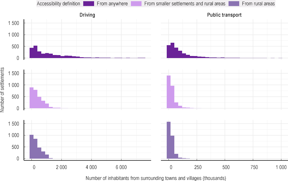
Figure 3.8 compares the three population accessibility measures for driving and public transport. Indeed, the measure of driving access is much greater than PTr access for all three measures. In some cases, especially for the “From anywhere” measure, the surrounding accessible population is much larger than the settlement’s own population (particularly if that settlement is a village).

Figure 3.8. Surrounding population measured with three accessibility definitions

Note: Each row in the figure corresponds to a different measure of accessible population from Table 3.1.

Source: Based on data from selected countries and regions.

Statlink

The analysis in this chapter tries to relate service provision in a settlement with how many people can potentially reach that settlement using public transport or driving. More than transport accessibility, a simple measure that sums the population that can reach the settlement within a certain time threshold may capture the number of people living in the surrounding areas of settlements, which is often related to the size of the settlement. For instance, larger settlements are more likely to be surrounded by dense areas (e.g. suburbs) than smaller settlements. If this is the case, towns would systematically have better accessibility than villages, independent of available transport links. To control for the population in the surrounding area, the analysis calculates a transport performance ratio following a similar approach to that used for transport accessibility in cities (ITF, 2019[2]). The numerator is how many people can reach the settlement within 45 minutes (under the 3 definitions of population in surrounding areas listed in Table 3.1) by driving or public transport. The denominator is how many people live within a 45 km radius of the settlement.4

To allow for comparability across all cases, this radius is drawn in the same way for all settlements and it is a perfect circle that does not depend on the transport mode. The transport performance ratio captures the effectiveness of the transport mode (car driving or PTr) in enabling access for people living in the surrounding area. If the ratio is large, the local public transport or road networks allow a greater fraction of people living around a settlement to reach it. Box 3.2 explains some ways transport accessibility metrics can be used to promote sustainable and equitable cities and communities.

What is the relationship between how readily people can reach a settlement and the provision of services in that settlement? Figure 3.9 plots the number of POIs in each settlement relative to the transport performance ratio (based on the “From smaller settlements and rural areas” measure). The relationship for public transport seems broadly positive, especially for towns. For driving, the relationship appears weakly negative. An econometric analysis like that in Chapter 2 can help understand the relationship between the population with access to a settlement (by driving or public transport) and its provision of services while controlling for other factors that may influence service provision, such as access to cities.

Figure 3.9. Relationship between the number of POIs and transport performance ratio

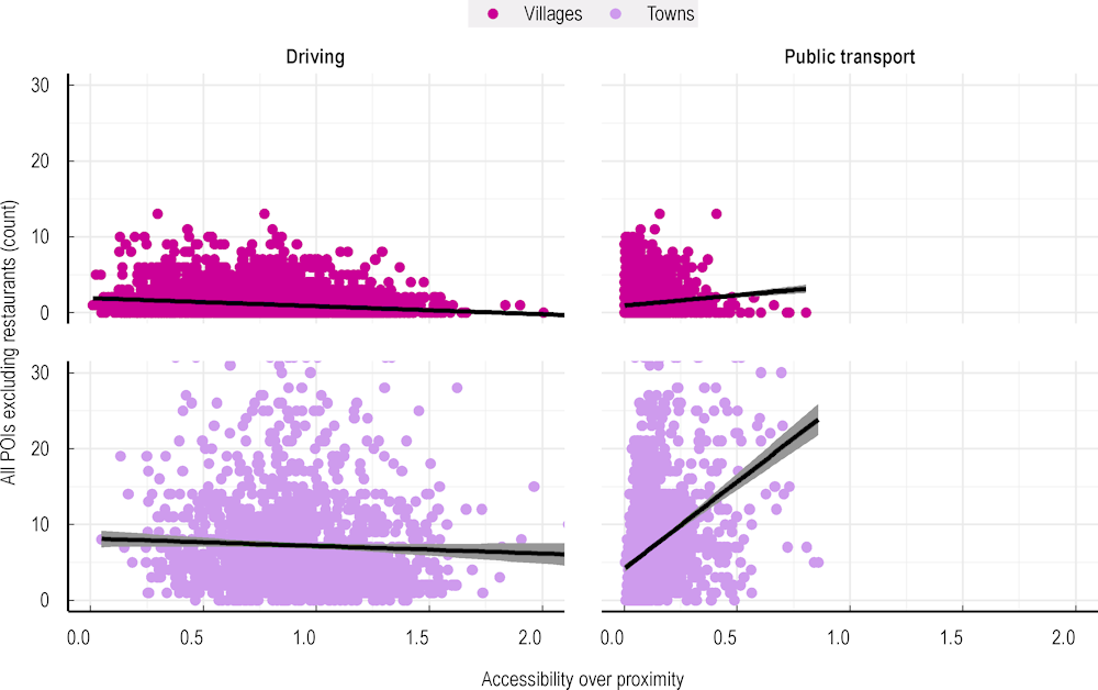
Note: Transport performance population ratio based on the “From smaller settlements and rural areas” measure. The ratio is the number of people that can access the settlement by PTr or within a 45‑minute drive (from outside any settlement or from smaller settlements) relative to the number of people living 45 km from the settlement border. In other words, it measures accessible population over proximate population.

Source: Based on data from selected countries and regions.

Statlink

Box 3.2. Transport and Sustainable Development Goals

The United Nations Sustainable Development Goal (SDG) 11 focuses on Sustainable cities and communities. Within this goal, the United Nations suggests that countries produce Indicator 11.2.1, measuring the proportion of people with convenient access to public transport by gender, age and disability status. The following dimensions are relevant for determining how many people have access to public transport based on their demographic characteristics:

• Type of public transport system (low-capacity such as buses vs. high-capacity such as trains).

• Travel mode that can be used to reach public transport, including active modes such as walking or biking within certain time or distance thresholds.

• Gender, age and disability status (considering physical and non-physically-limiting disabilities).

• Other dimensions include average household income, type of location (urban, suburban, rural) and transport infrastructure quality or performance.

Source: U.S. Government (2016[11]), “Indicator 11.2.1: Proportion of population that has convenient access to public transport, by sex, age and persons with disabilities”, https://sdg.data.gov/11-2-1/.

Regional centres

It is expected that regional centres (RCs), with their larger populations and greater variety of services, provide more services to people in surrounding areas. This chapter follows the method described in Chapter 1 to define RCs. In the transport sample, a total of 166 smaller settlements are RCs (Table 3.2). More towns than villages are RCs across all time thresholds. For example, within a 30-minute drive, 12% of towns are RCs (the largest reachable settlement) compared to only 3% of villages. As expected, RCs are much farther from cities than non-RCs (Annex Table 3.A.4).

Table 3.2. Share of villages, towns and cities that are regional centres

Settlement type	RC		Not an RC
	Number	%	Number	%
Villages	68	3.3	1 967	96.7
Towns	98	12.2	708	87.8
Cities	33	37.1	56	62.9

Source: Authors’ elaboration, selected countries and regions.

Service provision: Public transport versus driving

To highlight the relationship between the availability of public transport and provision of services, regression analysis can be used to evaluate whether the effectiveness with which people access a settlement helps predict the number of services in the settlement. Access is measured using public transport and then compared to a similar measure with a car journey. Box 3.3 presents the econometric framework in more detail; the remainder of this section focuses on analysis results and Box 3.4 presents robustness checks.

Box 3.3. Regression models: Baseline and extensions

The regression specification from Chapter 2 can be modified to include an additional term that captures the population outside of a settlement that can access services in the settlement.1 The baseline model in Equation 3.1 adds the transport performance ratio within a certain travel time threshold using different transport modes (e.g. car or PTr multi-modal routes).

Equation 3.1. Baseline regression

$Y_i=\alpha +{\beta }_1\mathrm{l}\mathrm{n}\left(Po{p}_i\right)+{\beta }_2{\ln \left(Po{p}_i\right)}^2+{\beta }_{3}Reg\mathrm{ }Cen{t}_i+{\beta }_4\mathrm{l}\mathrm{n}\left(Po{p}_i\right)\mathrm{*}Reg\mathrm{ }Cen{t}_i+{\beta }_5\mathrm{l}\mathrm{n}(Po{p}_i{)}^2\mathrm{*}Reg\mathrm{ }Cen{t}_i+{\beta }_6{drive\mathrm{ }time\mathrm{ }to\mathrm{ }a\mathrm{ }city}_i+{\mathit{\beta }}_7\mathit{t}\mathit{r}\mathit{a}\mathit{n}\mathit{s}\mathit{p}\mathit{o}\mathit{r}\mathit{t}\mathit{ }\mathit{p}\mathit{e}\mathit{r}\mathit{f}\mathit{o}\mathit{r}\mathit{m}\mathit{a}\mathit{n}\mathit{c}\mathit{e}\mathit{ }\mathit{r}\mathit{a}\mathit{t}\mathit{i}{\mathit{o}}_{\mathit{i}}+{\epsilon }_i$

where $Y$ is the number of services in settlement $i$, $\alpha$ is an intercept, $Pop$ is the settlement’s population, $Reg Cent$ is a dummy indicating whether the settlement is a 30-minute RC, $Drive time to a city$ indicates travel (driving) time to the closest city and $\epsilon$ is the idiosyncratic error. Proximity to cities may matter because people are more likely to bypass towns and villages if they have a city nearby. The main coefficient of interest is ${\beta }_7$, the transport performance ratio. Different from Chapter 2, the main results use the total number of POIs based on the groups in Figure 3.5 (

Annex Figure 3.D.2 shows some service-specific regression results).

Table 3.3 outlines three extensions. The dependent variable is still the number of POIs within the settlement. The “Settlement type” extension interacts with the accessible population outside of a settlement with a variable indicating whether the settlement is a village rather than a town. The effect for villages is ${\beta }_7+{\beta }_8$ (the overall effect plus the village-specific effect), while the effect for towns is just ${\beta }_7$. Next, the “Surrounding services” extension considers whether more services outside the settlement alters the relationship between car accessibility and services inside the settlement. Services outside are measured as the number of POIs in the 45-minute isochrone around the settlement. Finally, the “Regional centre” extension considers whether population accessibility operates differently between RCs and non-RCs.

Table 3.3. Regression model extensions

Extension	Additional regression terms	Rationale/research question
Settlement type interaction with transport performance ratio	β7transport performance ratioi+β8transport performance ratioi*villagei	Whether the relationship between services and transport differs by settlement type between towns and villages
Surrounding services measured as total POIs inside the 45-minute isochrone	β7transport performance ratioi+β8POIs in the surrounding area	Whether more availability of services outside settlements means people living outside do not need to travel to the settlement to access services
Regional centre interaction with transport performance ratio	β7transport performance ratioi+β8transport performance ratioi*RegCenti	Whether the relationship between services and transport differs by RCs and non-RCs

All of these regressions can reveal correlations only and not causality. Variables such as income or demographic composition, which are not included in the models (omitted variables), might impact the demand and supply of services (and thus the dependent variable). For example, places with better public transport might have more services because more people can get to them via transport or there could be reverse causality because the places the same with good provision of transport may also provide more public services like schools and hospitals (Székely and Novotný, 2022[12]).

1. The strong positive relationship between a settlement’s population and the total number of services available found in Chapter 2 is also verified for the sample of countries/regions in this chapter (Annex Table 3.D.3).

Source: Székely, V. and J. Novotný (2022[12]), “Public transport-disadvantaged rural areas in relation to daily accessibility of regional centre: Case study from Slovakia”, https://doi.org/10.1016/j.jrurstud.2022.03.015.

Settlements with better public transport accessibility have more services

Places with better public transport connections may have more services available. When using “All POIs (including restaurants)” as a dependent variable, the results of estimating Equation 3.1 indicate that settlements with more transport accessibility have a lower presence of services. When restaurants are excluded, better transport has a positive relationship with the availability of health, finance and education services (Figure 3.10). In other words, except for the dependent variable including restaurants, the results indicate that the population living in smaller settlements or rural areas outside the settlement that can access it via public transport has an additional positive (although small) effect on service provision inside, controlling for the size of a settlement’s own population.5

Using the “From smaller settlements and rural areas” definition, a 10% increase in the transport performance ratio is associated with a 0.4% increase in the expected number of “All POIs excluding restaurants” in the settlement. On average, settlements in the sample have a transport performance ratio of 0.098 for PTr, which means that nearly 10% of people living in a 45 km radius buffer around a settlement of interest (those in smaller settlements and rural areas) can access the settlement within 45 minutes.

Figure 3.10. Regression results for public transport, transport performance ratio coefficient

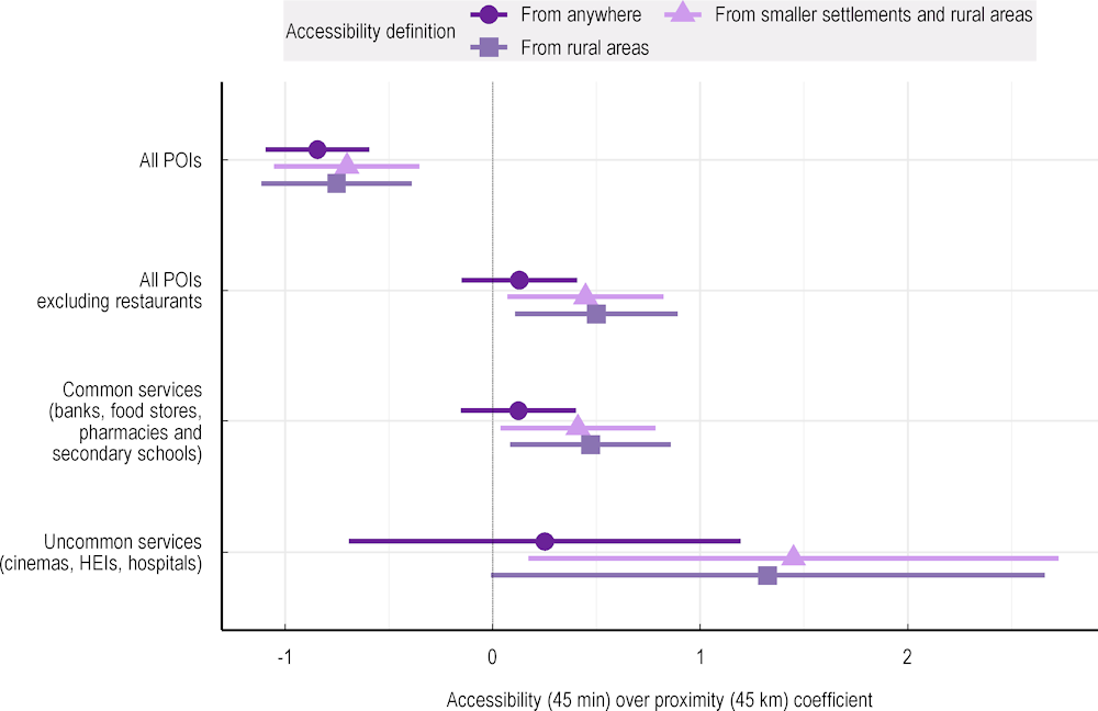
Note: ${\mathrm{\beta }}_7$ coefficient results based on the different accessibility measures from Table 3.1. Circles, triangles and squares represent point estimates, while bars represent a 95% confidence interval. Y-labels indicate different dependent variables. The “Uncommon services” model is estimated with logit, while the first three specifications use negative binomial regressions as they are suitable for zero-inflated count data. A more positive estimated coefficient corresponds to a higher expected number of POIs (log scale).

Source: Based on data from selected countries and regions.

Statlink

Settlements with better driving access have fewer services

Unlike public transport, which usually stops in smaller settlements, roads often connect large settlements to each other while bypassing smaller settlements. Thus, with better car accessibility, people looking for a wider range of higher-quality services might travel farther to larger settlements and, in the process, bypass smaller settlements with less choice in terms of types, prices and quality of services. In fact, the reduction in local service provision with better car access and the increasing concentration of retail activity in larger urban centres has been documented in the United Kingdom (Powe and Shaw, 2004[13]).

The econometric results show that regardless of POI measure (and even when considering the accessible population instead of the transport performance ratio), surprisingly, better driving access correlates with fewer services in towns and villages (Figure 3.11). These are the opposite findings from public transport accessibility. On average and using the “From smaller settlements and rural areas” definition, settlements in the sample have a transport performance ratio of 0.98 for driving, which means that nearly everyone living in a 45 km radius buffer around a settlement of interest (those in smaller settlements and rural areas) can access the settlement within 45 minutes. The corresponding estimates imply that a 10% increase in the transport performance ratio is associated with a 7% decrease in the expected number of services (“All POIs excluding restaurants”) in the settlement.

Figure 3.11. Regression results for driving, transport performance ratio

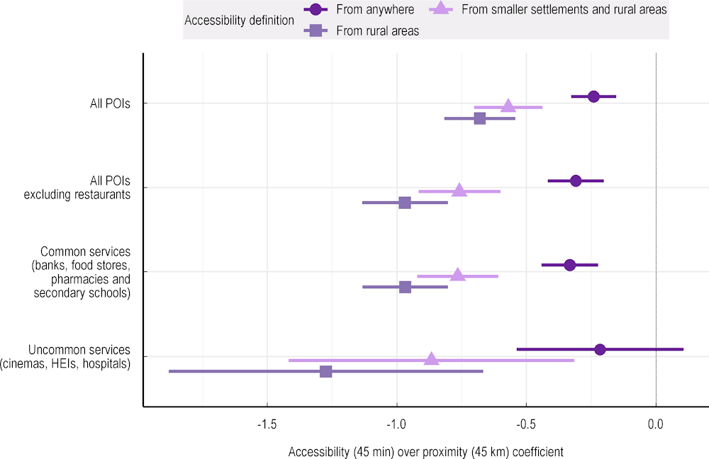
Note: ${\mathrm{\beta }}_7$ coefficient results using the population count “From smaller settlements and rural areas”. Circles, triangles and squares represent point estimates, while bars represent a 95% confidence interval. Y-labels indicate different dependent variables. The “Uncommon services” model is estimated with logit, while the first three specifications use negative binomial regressions as they are suitable for zero-inflated count data. A more positive estimated coefficient corresponds to a higher expected number of POIs (log scale).

Source: Based on data from selected countries and regions.

Statlink

Public transport accessibility is more beneficial for towns while driving accessibility has a more negative impact on villages

The relationship between the number of services and the accessibility of the surrounding population might differ between towns and villages (see Table 3.3). Towns, being larger, often have different functional roles and therefore provide a larger variety of services. Villages may mostly serve their local population while depending on nearby towns and cities for more specialised and diverse services. Thus, villages that have better accessibility are not necessarily more likely to serve people living in surrounding areas.

The results show that public transport relates positively to service provision in towns (Table 3.4). Villages instead show a slightly negative association between public transport accessibility and service provision. This implies that towns drive the positive relationship between public transport and services, as measured in the baseline model of all smaller settlements.

Cars show a negative association between driving accessibility and services, as before, but the negative relationship is twice as large for villages as for towns (Table 3.4). This may be because when smaller settlements (especially villages) are more accessible by car, they are more easily bypassed in favour of larger settlements while allowing the local population to go somewhere else more easily. Thus, better car accessibility around villages is especially detrimental to their provision of services.

Table 3.4. Transport performance ratio regression estimates for villages and towns

	Public transport	Driving
Villages	Small negative effect (-0.2)	Large negative effect (-1.1)
Towns	Large positive effect (0.7)	Moderate negative effect (-0.5)

Note: ${\mathrm{\beta }}_7$ and ${\mathrm{\beta }}_7$+${\mathrm{\beta }}_8$ coefficient results using the population count “From smaller settlements and rural areas” with “All POIs excluding restaurants”.

Source: Based on data from selected countries and regions. Full results are available in Annex Table 3.E.1.

The negative effect of driving on service provision in the settlement is unaffected by the number of services outside the settlement

Given good connectivity, people may not care whether a service is provided inside or outside a settlement (e.g. people going out to eat in a rural area may be indifferent between a roadside restaurant or one in a village). Driving accessibility could be negatively related to services inside the settlement because more accessibility could increase the attractiveness (and substitutability) of services outside the settlement.

The results show that driving accessibility is still negatively related to POIs in the settlement even when accounting for POIs in the outside isochrone (Annex Table 3.E.2). Controlling for the supply of services outside does not change the negative effect of driving accessibility on services inside settlements. In fact, it actually makes the effect slightly more negative (from -0.76 to -0.81). In addition, settlements with more services in their hinterlands also have more services inside their boundaries.6 Therefore, services outside might capture the economic structure of the surrounding area, e.g. places with higher income might have more services both in the hinterland and inside settlements.

While car accessibility is associated with more services in regional centres, public transport accessibility is not

Chapter 2 finds that larger, more central settlements like RCs have more services than settlements of the same size that are not RCs. Thus, towns and villages that are RCs play particularly important roles in providing services to the population in their surrounding areas.

The results confirm that driving accessibility boosts services in these RCs. In other words, RCs appear to benefit more from car accessibility than smaller settlements: car-accessible RCs have more services than car-accessible non-RCs. However, driving still has a negative effect overall on services even in RCs but the negative effect of driving is weaker (less negative) for RCs compared to non-RCs (Annex Table 3.E.3).

For PTr-accessible RCs, the results indicate the opposite effect. In other words, the effect of greater public transport accessibility on services is negative in RCs compared to a positive effect for non-RCs.7 As the baseline results indicated a positive relationship between public transport and service provision, this positive relationship seems to come from settlements that are not RCs.

Box 3.4. Robustness checks

Figure 3.12 summarises results for the measure of transport accessibility (transport performance ratio coefficient) for both cars and PTr from the baseline and model extensions. They rely on the “From smaller settlements and rural areas” definition to measure accessible population (see Table 3.1). The dependent variable uses “All POIs excluding restaurants” since restaurants are plentiful and can overwhelm the counts of other services. As indicated by the figure, the main results are relatively stable across the different model extensions and all point in the same direction for POIs: there is a positive effect on public transport and a negative effect on car accessibility.

Figure 3.12. Regressions results for “All POIs excluding restaurants”

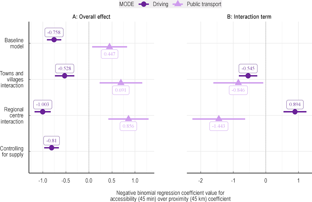
Note: ${\mathrm{\beta }}_7$ and ${\mathrm{\beta }}_8$ (when applicable) coefficient results of Equation 3.1 and model extensions (Table 3.3) using the “From smaller settlements and rural areas” population count and taking the set of “All POIs excluding restaurants” as the dependent variable. Circles and triangles represent point estimates, while bars represent a 95% confidence interval. Y-labels indicate different regression models. Models were estimated using negative binomial regressions as they are suitable for zero-inflated count data.

Source: Based on data from selected countries and regions.

Statlink

Conclusions

The analysis in this chapter explores the relationship between service provision and transit accessibility, specifically for towns and villages. It considers both car and public (multimodal) transport access measures in multiple countries. It generally finds that better PTr accessibility from the area around a settlement has a positive relationship with services inside the settlement. The positive correlation between services and PTr access is more pronounced for towns, especially those that are not RCs. Conversely, improved driving access is associated with fewer services in the settlement itself, especially if the settlement is a village. The negative effect of driving on service availability remains consistent regardless of the number of POIs outside the settlement, yet it is slightly smaller for RCs.

Expanding public transport to towns can boost well-being, especially for people without access to cars, because service provision in towns is positively related to PTr access. Better PTr access can also improve the emissions profile associated with frequent travel. The data show that better car accessibility could, however, result in villages and being bypassed for larger settlements. This is not surprising: OECD analysis shows that policies targeting infrastructure and road connectivity are not by themselves the most effective tools for strengthening small and remote regions. Instead, policies targeting infrastructure and road connectivity should be strategic and co-ordinated with broader rural and regional policies (OECD, 2012[5]).

Annex 3.A. Additional data information

Annex Table 3.A.1– Annex Table 3.A.3 describe the additional services and display summary statistics for the sample of five countries and one region used throughout the chapter.

Annex Table 3.A.1. Description of services included in the analysis

Name	Service	Category	Included	Excluded
Cinemas	Cinemas	Commercial	Theatres showing movies.
Food stores	Food stores	Commercial	Independent and chain retail stores selling food (e.g. supermarkets and convenience stores).	Small produce stores or specialised food stores.
Restaurants	Restaurants and bars	Commercial	Independent and chain restaurants and bars.

Annex Table 3.A.2. Number of cities, towns and villages in selected countries and regions

Country/region	Cities	Towns	Villages	Total
Estonia	3	20	79	102
Luxembourg	1	19	55	75
Netherlands	50	328	636	1 014
Sardinia, Italy	2	48	235	285
Sweden	17	213	574	804
Switzerland	16	178	456	650
Total	89	806	2 035	2 390

Source: Based on sources in Annex Table 1.A.3 and on data from selected countries and regions.

Annex Table 3.A.3. Population of cities, towns and villages in selected countries and regions

Settlement type	Minimum	Median	Mean	Maximum
Villages	250	1 284	1 652	4 991
Towns	700	8 498	12 212	49 239
Cities	51 667	92 695	177 577	1 384 868

Source: Based on sources in Annex Table 1.A.3 and on data from selected countries and regions.

Annex Table 3.A.4 shows the distribution of driving time to a city by settlement type, separating RCs from non-RCs. For villages, non-RCs are an average of 45 minutes away from a city, while the median RC village is at least 2 hours away from a city (the upper limit). For towns, non-RCs average only 25 minutes away from a city, while for RCs average at least 1.5 hours from a city.

Annex Table 3.A.4. Driving time to a city in minutes, by settlement type and RC status

Settlement type	Minimum	Median	Mean	Maximum
Villages: Not RCs	0.77	30.0	45.7	120
Villages: RCs	39.5	120	104.0	120
Towns: Not RCs	3.31	17.7	25.9	120
Towns: RCs	27.2	120	90.8	120

Note: Travel times are capped at 120 minutes. Means include all values that are top-coded 120 minutes.

Source: Based on data from selected countries and regions.

Annex 3.B. Data sources and processing for accessibility measures

Travel times by car are calculated using shortest-path algorithms available in the open-source GeoDMS software and data from network topology and maximum speeds encoded for in-car navigation from TomTom/OSM data (TomTom, 2018[14]).

Public transport times rely on GTFS data. The GTFS is an open and standardised format used by transit agencies around the world to distribute information about their public transport networks. They contain multiple files with information about routes, trips, schedules, fares and the exact geographic details of each transit station and stop.

Annex Table 3.B.1 provides the data sources and managing agencies for each country included in the study. Verification exercises confirmed that the transport sample of five countries and one region all have comprehensive public transport data. This type of GTFS data is continually improving; thus, applying a similar method to a larger sample of countries in the future should be possible. To increase comparability between countries, a representative weekday in September 2023 was chosen for routing. The common day was not a holiday and appears in as many of the retrieved GTFS schedules as possible. According to these schedules, more than 90% of settlements in the sample, including small villages, have at least some form of available public transport.

Annex Table 3.B.1. GTFS information by country/region

Country	Managing agency	Website	Download date	Routing reference date
Estonia	Estonian Transport Administration	http://peatus.ee/gtfs/gtfs.zip	29/08/2023	06/09/2023
Luxembourg	Administration des transports publics	https://download.data.public.lu/resources/horaires-et-arrets-des-transport-publics-gtfs/20230823-081943/gtfs-20230822-20230909.zip	29/08/2023	06/09/2023
Netherlands	OpenGeoHub Foundation	https://gtfs.ovapi.nl/nl/gtfs-nl.zip	30/10/2023	09/11/2023
Sweden	Trafiklab	https://www.trafiklab.se/api/trafiklab-apis/gtfs-sverige-2/static-data/	29/08/2023	07/09/2023
Switzerland	Federal Roads Office FEDRO	https://opentransportdata.swiss/en/dataset/timetable-2023-gtfs2020/resource/69b41a1a-6fa4-4cfa-b38f-ac2cfa428276	29/08/2023	14/09/2023
Sardinia, Italy	Regione Autonoma della Sardinia	https://www.dati.gov.it/view-dataset?Cerca=Quadri+orari ARST: http://arstspa.info/arst-cagliari-it.zip ASPO: https://www.aspo.it/ ATP Nuoro: https://www.atpnuoro.it/media/files/dati_atpnu.zip ATP Sassari: https://atpsassari.it/media/files/atpss-gtfs.zip CTM: https://www.ctmcagliari.it/open_data/GTFS.zip Private: http://www.sardegnamobilita.it/opendata/dati_privati.zip Traghetti: http://www.sardegnamobilita.it/opendata/dati_mare.zip Trenitalia: http://www.sardegnamobilita.it/opendata/dati_trenitalia.zip	29/08/2023	13/09/2023

Source: Based on Mobility Database (2024[15]), Homepage, https://mobilitydatabase.org/, Accessed 22 February 2024.

The European Commission Joint Research Centre developed the public transport routing tool used to find viable schedules and route combinations in collaboration with the Università degli Studi di Pavia. The core algorithm of this tool, called VelociRAPTOR, is based on the RAPTOR algorithm described by Delling, Pajor and Werneck (2014[16]). The tool is particularly efficient in its computational and memory performance when handling large-scale public transport queries. This is particularly important when searching for optimal trips over dense public transport networks between many origins and destinations.

To reduce computational and analytic complexity, the set of destinations is the entire settlement rather than specific service points. It is assumed that once a commuter arrives at the settlement, s/he may access any of its local services. However, settlements are not represented as one destination point in their centre. Instead, all grid cells within a settlement are considered possible destinations. This has the advantage that the measured settlement accessibility does not depend on the chance connectivity characteristics of a given suburb to the settlement’s geographic centre. The downside is that every considered origin point can have multiple valid destinations within the same settlement, with slightly varying travel times.

Annex 3.C. Method for calculating accessibility

This section describes a method for calculating the three measures of accessible population (“From anywhere”, “From smaller settlements and rural areas”, “From rural areas”) and illustrates various examples. Since the method seeks to establish a single travel time value for a settlement’s accessibility from outside, it requires that travel time matrices reflect a single travel time between each origin grid cell and destination settlement (which are all composed of one or more grid cells). When there are multiple destination grid cells $k$ in a settlement, the representative travel time from the non-settlement grid cell to the settlement is the minimum travel time between the centroid of each origin grid cell and the centroid of any grid cell within the destination settlement. For example, a traveller coming from the north periphery of a city will often arrive most quickly in the northern part of the city first and use services in the part of the settlement most accessible to them.

Formally, suppose there is a matrix of inhabited 1 km² grid cells. Each grid cell has three indices indicating whether it belongs to a settlement or not ($s=\{<!--\; -->\mathrm{0,1}\}$) and, if $s=1$ (grid cell belongs to a settlement), the settlement’s unique code is ordered by settlements’ hierarchy ($i=1, \dots ,S$ for the origin settlement and $j=1,\dots , S$ for the destination settlement). If $s=0$, the grid cell has a unique identifier, $i$ ($i=1, \dots ,S$). The number of inhabitants is indicated by $P_{s,i,k}$, with $i$ indicating the list of origins and $k$ the cell number within the settlement ($k=1,\dots K$).

Travel times are stored in two separate matrices $T_{i,j}^m$, indicating travel times between origins $i$, and destination grid cells $j$, depending on travel mode $m$ (driving with a car and taking multimodal public transport). The travel time isochrone of settlement destination $j$ is the minimum of all travel time matrices that could reach any grid cell that belongs to $j$. If $T_{i,k;j}<t$, then the grid cell population is considered. Accessibility for the “From anywhere” definition is:

Equation 3.2. From anywhere population equation

$A_j^m\left(t\right)=\sum _{s=0}^1\sum _{i=1}^S\sum _{k=1}^K\left(T_{i,k;j}<t\right)*P_{s,i,k} , \forall i\ne j$

Summing the population from lower hierarchical level settlements gives the definition for the population “From smaller settlements and rural areas”:

Equation 3.3. From smaller settlements and rural areas population equation

$A_j^m\left(t\right)=\sum _{s=0}^1\sum _{i=1}^S\sum _{k=1}^K\left(T_{i,k;j}<t\right)*P_{s,i,k} , \forall i<j$

Finally, if $s=0$, the definition of population outside settlements living in rural areas is:

Equation 3.4. From rural areas population equation

$A_j^m\left(t\right)=\sum _{i=1}^S\sum _{k=1}^K\left(T_{i,k;j}<t\right)*P_{0,i,k} , \forall i\ne j$

Below is a graphical representation of the accessibility indicator calculations for the 3-by-3 grid cell settlement in the middle of the figure for a 45-minute drive. It is said to be $j=2$ because it has second level hierarchy in the settlements in its country. All other numbers in black circles indicate other settlements’ hierarchical position in the country’s network of settlements. Departing from each grid cell of settlement $j\ne 2$ yields travel time estimates to all grid cells of settlement $j=2$.

Notably, settlements are not represented as single centroids or specific central destination points, which makes the approach very sensitive to chance connectivity characteristics. For example, in Europe, public transport terminals and main road thoroughfares are often constructed outside medieval city centres and settlement centres are often relatively poorly connected. Instead, with this analytical approach, destinations can be any grid cell within the settlement’s boundaries. The travel time between grid cells outside the settlement will be the minimum travel time to any cell of the settlement.

Annex Figure 3.C.1. Accessibility measures: Travel time

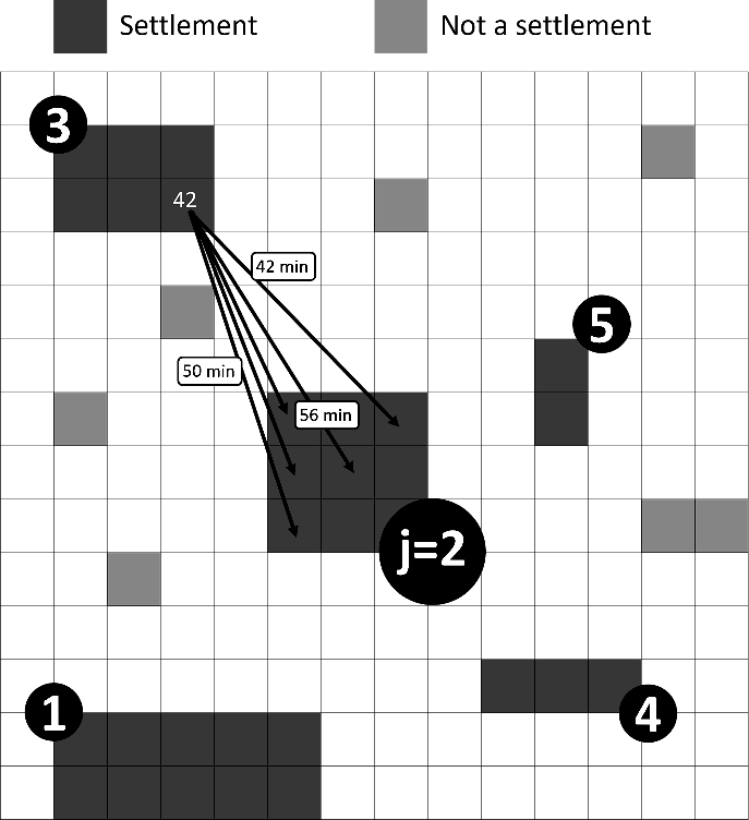
The settlement’s final travel time matrix isochrone (represented by the solid curve) is the minimum travel time between all grid cells outside the settlement and any grid cell inside the settlement. All grid cells inside the solid line can reach the settlement $j=2$ within a 45-minute drive.

Annex Figure 3.C.2. Accessibility measures: Minimum travel time isochrone

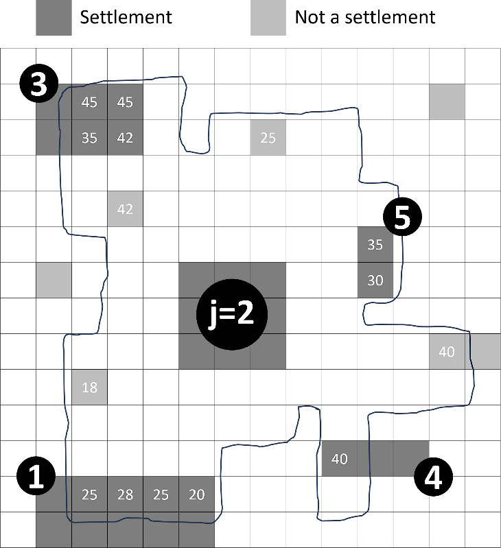
Now that the travel time isochrone is defined, a population that can access the settlement are summed over $j=2$.

Annex Figure 3.C.3. Accessibility measures: Minimum travel time isochrone, cell indexes

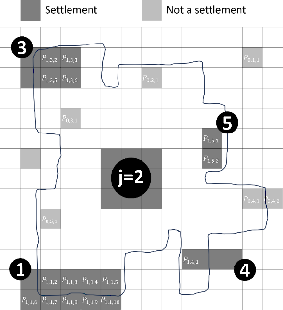
The “From anywhere” definition sums all inhabited grid cells inside the travel time isochrone.

Equation 3.5. Sum of population for the From anywhere population measure

$A_2^m=P_{\mathrm{0,2},1}+P_{\mathrm{0,3},1}+P_{\mathrm{0,4},1}+P_{\mathrm{0,5},1}+P_{\mathrm{1,1},2}+P_{\mathrm{1,1},3}+P_{\mathrm{1,1},4}+P_{\mathrm{1,1},5}+P_{\mathrm{1,3},2}+P_{\mathrm{1,3},3}+P_{\mathrm{1,3},5}+P_{\mathrm{1,3},6}+P_{\mathrm{1,4},1}+P_{\mathrm{1,5},1}+P_{\mathrm{1,5},2}$

See that grid cells 1,1,6 and 0,4,2 are not considered because they are outside the travel time isochrone of settlement $j=2$. If the settlement of interest is positioned second in the hierarchy, only the population from the settlement $i>2$ is summed, that is, the population from the settlement $i=1$ is excluded. Therefore:

Equation 3.6. Sum of population for the From smaller settlements and rural areas measure

$A_2^m=P_{\mathrm{0,2},1}+P_{\mathrm{0,3},1}+P_{\mathrm{0,4},1}+P_{\mathrm{0,5},1}+P_{\mathrm{1,3},2}+P_{\mathrm{1,3},3}+P_{\mathrm{1,3},5}+P_{\mathrm{1,3},6}+P_{\mathrm{1,4},1}++P_{\mathrm{1,5},1}+P_{\mathrm{1,5},2}$

The Outside population definition is:

Equation 3.7. Sum of population for the From rural areas measure

$A_2^m=P_{\mathrm{0,2},1}+P_{\mathrm{0,3},1}+P_{\mathrm{0,4},1}+P_{\mathrm{0,5},1}+P_{\mathrm{1,1},2}$

Annex Table 3.C.1 presents the surrounding population accessibility measures in descending order of restrictiveness using a 45-minute travel time threshold to villages and towns by car and PTr. “From smaller settlements and rural areas” have a greater maximum than the “From rural areas” measure, indicating that smaller settlements can add considerably to the accessible population both by car and PTr. However, larger settlements are still more pivotal, as the “From smaller settlements and rural areas” measure is closer to the “From rural areas” measure than the “From anywhere” population measure.

Annex Table 3.C.1. Population around towns and villages

Population measure	Minimum	Median	Mean	Maximum
A. Car
From anywhere	1 231	889 623	1 503 088	9 709 076
From smaller settlements and rural areas	1 231	286 317	411 349	4 298 016
From rural areas	1 231	229 808	330 623	1 331 700
B. Public transport
From anywhere	0	56 259	113 204	1 547 151
From smaller settlements and rural areas	0	14 429	27 518	499 870
From rural areas	0	12 032	20 458	277 223

Note: Seven villages in Italy and one village in Sweden do not have public transport networks; thus, their accessible surrounding PTr population is zero (minimum values in Panel B).

Source: Based on sources in Annex Table 1.A.3 and on data from selected countries and regions.

Annex 3.D. Regression equations and methods

As in Chapter 2, a negative binomial equation is used to model the relationship between common services in a settlement and the settlement’s population. Usually, researchers use a Poisson model to model count data. Nevertheless, in the Poisson distribution, the mean ($\mathrm{{\rm E}}\left(Y\right)=\mu$) must be equal to the variance ($\mathrm{V}\mathrm{a}\mathrm{r}\left(Y\right)=\mu$), which is not the case in the transport sample data (see Annex Table 3.D.1). Because of the excess zeros, the variance of the data becomes much larger than the mean, a phenomenon called overdispersion. In these cases, the negative binomial model is preferred because it accounts for the overdispersion in the variance, correcting standard errors.

Annex Table 3.D.1. Average and variance in the number of POIs, selected countries and regions

Variable	Average number of POIs per settlement	Variance in the number of POIs per settlement	Overdispersion: p-value from t-test
All POIs excluding restaurants	2.84	25.22	0.000
Common services (excluding restaurants)	2.33	15.57	0.000
Restaurants	10.26	410.50	0.000

Note: A test for overdispersion checks the assumption of $E\left(Y\right)=\mu =Var\left(Y\right)$ (null hypothesis) against the alternative that $Var\left(Y\right)=\mu +c*f\left(\mu \right)$. The third column presents the p-value for the t-test of $H_0:c=0$ versus $H_1:c\ne 0$. If the p-value is smaller than 0.05, $H_0$ is rejected and we cannot confirm that the variance is equal to the mean.

Source: Based on data from selected countries and regions.

Similar to Chapter 2, a logit equation is used for uncommon services to model whether a settlement has at least one cinema, hospital or HEI (such as a university). However, the logit model presents two challenges in the transport sample: separation and rare events. Separation occurs when the outcome variable separates a predictor variable completely. For example, if hospitals are only located in RCs, the RC variable perfectly predicts the existence of hospitals. Thus, the Likelihood for the RC coefficient cannot be estimated. Separation makes it impossible to compute the coefficient for the predictor variable causing the separation but it does not interfere with other variables’ estimates. Moreover, the well‑established Firth model, or penalised maximum likelihood estimation, generates finite and consistent estimates of regression parameters in cases of small samples and separation. On the other hand, rare events are more problematic. Logistic model maximum likelihood estimation suffers from small-sample bias. The small sample notion does not consider the full sample but the number of cases in the less frequent of the two categories. In the transport sample, fewer than 10% of smaller settlements have a hospital or a HEI. Therefore, estimating the likelihood of these services might result in biased estimators.

Annex Table 3.D.2. Hospitals and HEIs in villages and towns (selected countries and regions)

Group	Number of villages and towns	Percentage
Does not have a cinema, a hospital or an HEI	2 421	85.22
Has a cinema or a hospital or an HEI	420	14.78

Source: Based on data from selected countries and regions.

Baseline regression estimation

This section shows coefficients of Equation 3.1, estimated using a negative binomial model for the set of “All POIs excluding restaurants”. Coefficients are interpreted as changes in log counts and are analysed in terms of direction and magnitude. The estimated coefficient for the “Transport performance ratio” (highlighted in purple) is of particular interest. As discussed before, the transport performance coefficient is positive for public transport and negative for driving, regardless of the accessibility measure used to count population in the hinterland. The use of the “From smaller settlements and rural areas” or “From rural area” accessibility measure makes the coefficient larger (more negative or more positive) compared to the “From anywhere” measure.

Annex Table 3.D.3. Regression results of baseline model

Dependent variable: All POIs excluding restaurants

	Public transport			Driving
	From anywhere	From smaller settlements and rural areas	From rural areas	From anywhere	From smaller settlements and rural areas	From rural areas
Intercept	-10.15***	-10.16***	-10.13***	-9.72***	-9.12***	-8.89***
	(1.08)	(1.08)	(1.08)	(1.08)	(1.08)	(1.07)
Log(Pop)	1.57***	1.58***	1.57***	1.54***	1.47***	1.46***
	(0.26)	(0.26)	(0.26)	(0.26)	(0.26)	(0.26)
Log(Pop)²	-0.03**	-0.04**	-0.03**	-0.03*	-0.02	-0.02
	(0.02)	(0.02)	(0.02)	(0.02)	(0.02)	(0.02)
Reg Cent	9.28***	8.94***	8.88**	10.95***	12.59***	11.66***
	(3.48)	(3.47)	(3.47)	(3.44)	(3.38)	(3.36)
Log(Pop) * Reg Cent	-1.81**	-1.73**	-1.71**	-2.23***	-2.63***	-2.39***
	(0.81)	(0.81)	(0.81)	(0.80)	(0.79)	(0.78)
Log(Pop)² * Reg Cent	0.09*	0.08*	0.08*	0.11**	0.14***	0.12***
	(0.05)	(0.05)	(0.05)	(0.05)	(0.05)	(0.04)
Drive time	0.01***	0.01***	0.01***	0.01***	0.01***	0.01***
	(0.00)	(0.00)	(0.00)	(0.00)	(0.00)	(0.00)
Transport performance ratio	0.13	0.45**	0.50**	-0.31***	-0.76***	-0.97***
	(0.14)	(0.19)	(0.20)	(0.06)	(0.08)	(0.08)

* p < 0.10.

** p < 0.05.

*** p < 0.01.

Source: Based on Equation 3.1 for selected countries and regions.

Annex Table 3.D.1 presents the overall and interaction terms for different sets of services, using the “From smaller settlements and rural areas” accessibility measurement. Annex Table 3.D.2 uses a similar setup but presents results service by service.

Annex Figure 3.D.1. Regression results of baseline model, sets of services

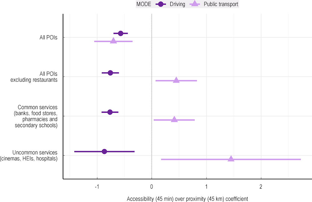
Note: ${\mathrm{\beta }}_7$ coefficient results based on Equation 3.1 using the “From smaller settlements and rural areas” population count. Circles and triangles represent point estimates, while bars represent a 95% confidence interval. Y-labels indicate different dependent variables. The “Uncommon services” model is estimated with logit, while the first 3 specifications use negative binomial regressions for zero-inflated count data.

Source: Based on data from selected countries and regions.

Statlink

Annex Figure 3.D.2. Regression results of baseline model, service by service

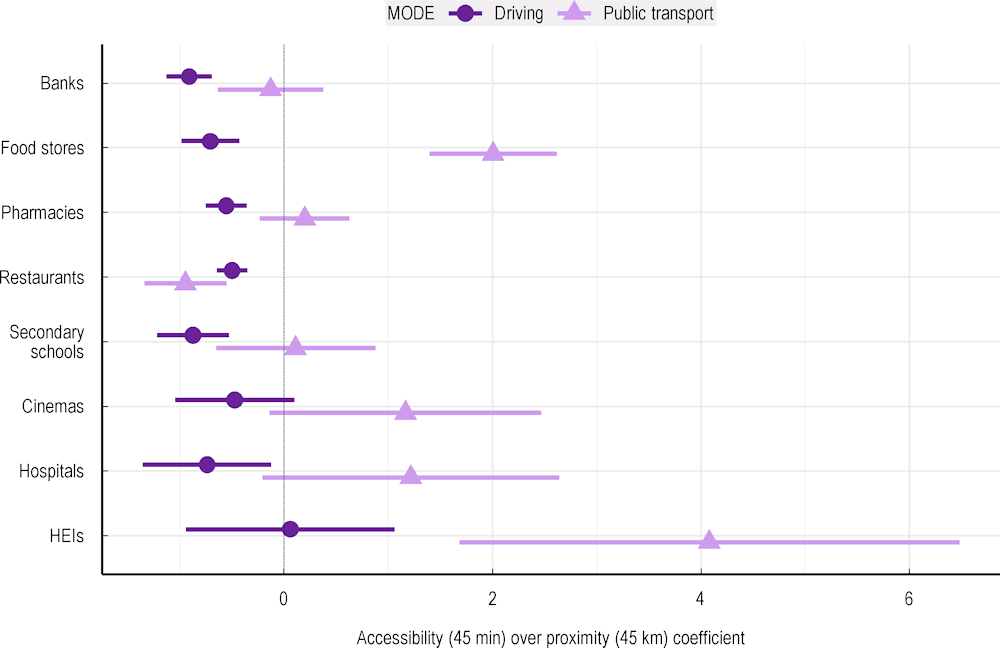
Note: ${\mathrm{\beta }}_7$ coefficient results based on Equation 3.1, using the “From smaller settlements and rural areas” population count. Circles and triangles represent point estimates, while bars represent a 95% confidence interval. Y-labels indicate different dependent variables. “Cinemas”, “Hospitals” and “HEIs” models are estimated with logit, while the first 5 specifications use negative binomial regressions for zero-inflated count data.

Source: Based on data from selected countries and regions.

Statlink

Annex 3.E. Results from model extensions – villages and towns

Annex Table 3.E.1 shows results from the regression for the set of POIs excluding restaurants. It interacts with the transport performance ratio as an indicator of whether a settlement is a village. Additional tables and graphs are available for the other dependent variables (including service-by-service) regressions. The estimated coefficients for the “Transport performance ratio” (highlighted in purple) are of particular interest.

Regression model including interaction for settlement type

$Y_i^s=\alpha +{\beta }_1\ln \left(Po{p}_i\right)+{\beta }_2{\ln \left(Po{p}_i\right)}^2+{\beta }_{3}Reg Cen{t}_i+{\beta }_4\ln \left(Po{p}_i\right)*Reg Cen{t}_i+{\beta }_5{\ln \left(Po{p}_i\right)}^2*Reg Cen{t}_i+{\beta }_6{drive time}_i+{\beta }_{7}transport performance rati{o}_i+{\mathit{\beta }}_8\mathit{t}\mathit{r}\mathit{a}\mathit{n}\mathit{s}\mathit{p}\mathit{o}\mathit{r}\mathit{t}\mathit{ }\mathit{p}\mathit{e}\mathit{r}\mathit{f}\mathit{o}\mathit{r}\mathit{m}\mathit{a}\mathit{n}\mathit{c}\mathit{e}\mathit{ }\mathit{r}\mathit{a}\mathit{t}\mathit{i}{\mathit{o}}_{\mathit{i}}\mathit{*}\mathit{v}\mathit{i}\mathit{l}\mathit{l}\mathit{a}\mathit{g}{\mathit{e}}_{\mathit{i}}+{\epsilon }_i$

Annex Table 3.E.1. Regression results of villages interaction model

Dependent variable: All POIs excluding restaurants

	Public transport			Driving
	From anywhere	From smaller settlements and rural areas	From rural areas	From anywhere	From smaller settlements and rural areas	From rural areas
Intercept	-9.61***	-9.78***	-9.73***	-9.66***	-9.02***	-8.61***
	(1.11)	(1.11)	(1.11)	(1.11)	(1.12)	(1.13)
Dummy village	1.54***	-0.12	-0.11	1.61***	0.28*	0.17
	(0.26)	(0.08)	(0.08)	(0.26)	(0.16)	(0.16)
Log(Pop)	-0.04**	1.59***	1.57***	-0.04***	1.53***	1.48***
	(0.02)	(0.26)	(0.26)	(0.02)	(0.26)	(0.26)
Log(Pop)²	10.59***	-0.04***	-0.04**	11.82***	-0.03**	-0.03**
	(3.46)	(0.02)	(0.02)	(3.40)	(0.02)	(0.02)
Reg Cent	-2.12***	10.65***	10.66***	-2.44***	12.85***	12.30***
	(0.81)	(3.46)	(3.45)	(0.79)	(3.36)	(3.34)
Log(Pop) * Reg Cent	0.11**	-2.10***	-2.10***	0.13***	-2.70***	-2.57***
	(0.05)	(0.81)	(0.80)	(0.05)	(0.78)	(0.78)
Log(Pop)² * Reg Cent	0.01***	0.10**	0.10**	0.01***	0.14***	0.13***
	(0.00)	(0.05)	(0.05)	(0.00)	(0.05)	(0.04)
Drive time	0.26	0.01***	0.01***	-0.15**	0.010***	0.01***
	(0.18)	(0.00)	(0.00)	(0.06)	(0.00)	(0.00)
Transport performance ratio	-0.44	0.69***	0.80***	-0.55***	-0.53***	-0.75***
	(0.29)	(0.24)	(0.25)	(0.10)	(0.11)	(0.12)
Transport performance * Village	0.00	-0.85**	-1.02**	0.00	-0.54***	-0.45***
	0.00	(0.39)	(0.40)	0.00	(0.14)	(0.15)

* p < 0.10.

** p < 0.05.

*** p < 0.01.

Source: Based on data from selected countries and regions.

Results from model extensions: POIs in the surrounding area

Annex Table 3.E.2 shows results from including the number of POIs in the surrounding area as an additional control when estimating the model for driving. The estimated coefficient for the “Transport performance ratio” (highlighted in purple) is of particular interest.

Regression model controlling for services in the surrounding area

$Y_i=\alpha +{\beta }_1\ln \left(Po{p}_i\right)+{\beta }_2{\ln \left(Po{p}_i\right)}^2+{\beta }_{3}Reg Cen{t}_i+{\beta }_4\ln \left(Po{p}_i\right)*Reg Cen{t}_i+{\beta }_5{\ln \left(Po{p}_i\right)}^2*Reg Cen{t}_i+{\beta }_6{drive time}_i+{\beta }_{7}transportperformance rati{o}_i+{\mathit{\beta }}_8\mathit{P}\mathit{O}\mathit{I}\mathit{s}\mathit{ }\mathit{i}\mathit{n}\mathit{ }\mathit{t}\mathit{h}\mathit{e}\mathit{ }\mathit{s}\mathit{u}\mathit{r}\mathit{r}\mathit{o}\mathit{u}\mathit{n}\mathit{d}\mathit{i}\mathit{n}\mathit{g}\mathit{ }\mathit{a}\mathit{r}\mathit{e}\mathit{a}+{\epsilon }_i$

Annex Table 3.E.2. Regression results controlling for POIs in hinterlands

Dependent variable: All POIs excluding restaurants

	Driving
	From anywhere	From smaller settlements and rural areas	From rural areas
Intercept	-10.09***	-9.59***	-9.43***
	(1.08)	(1.07)	(1.07)
Log(Pop)	1.62***	1.58***	1.59***
	(0.26)	(0.26)	(0.25)
Log(Pop)²	-0.04**	-0.03**	-0.03**
	(0.02)	(0.02)	(0.02)
Reg Cent	11.28***	13.2***	12.29***
	(3.42)	(3.35)	(3.32)
Log(Pop) * Reg Cent	-2.32***	-2.8***	-2.57***
	(0.80)	(0.78)	(0.77)
Log(Pop)² * Reg Cent	0.12***	0.15***	0.14***
	(0.05)	(0.04)	(0.04)
Drive time	0.01***	0.01***	0.01***
	(0.00)	(0.00)	(0.00)
Transport performance ratio	-0.32***	-0.81***	-1.06***
	(0.06)	(0.08)	(0.09)
POIs in the surrounding area	0.0001***	0.0002***	0.0002***
	(0.0000)	(0.0000)	(0.0000)

* p < 0.10.

** p < 0.05.

*** p < 0.01.

Source: Based on data from selected countries and regions.

Results from model extensions: Regional centres

Annex Table 3.E.3 shows results from interacting with an indicator for whether a settlement is a 30-minute RC (or not) with the measure of transport performance. The overall effect is the coefficient for all villages and towns, and the interaction term is an extra effect for those settlements that are RCs.

Regression model including interaction for RCs

$Y_i=\alpha +{\beta }_1\ln \left(Po{p}_i\right)+{\beta }_2{\ln \left(Po{p}_i\right)}^2+{\beta }_{3}Reg Cen{t}_i+{\beta }_4\ln \left(Po{p}_i\right)*Reg Cen{t}_i+{\beta }_5{\ln \left(Po{p}_i\right)}^2*Reg Cen{t}_i+{\beta }_6{Drive time}_i+{\beta }_{7}transport performance rati{o}_i+{\mathit{\beta }}_8\mathit{t}\mathit{r}\mathit{a}\mathit{n}\mathit{s}\mathit{p}\mathit{o}\mathit{r}\mathit{t}\mathit{ }\mathit{p}\mathit{e}\mathit{r}\mathit{f}\mathit{o}\mathit{r}\mathit{m}\mathit{a}\mathit{n}\mathit{c}\mathit{e}\mathit{ }\mathit{r}\mathit{a}\mathit{t}\mathit{i}{\mathit{o}}_{\mathit{i}}\mathit{*}\mathit{R}\mathit{e}\mathit{g}\mathit{C}\mathit{e}\mathit{n}{\mathit{t}}_{\mathit{i}}+{\epsilon }_i$

Here, ${\beta }_7$ is the overall effect for all settlements and ${\beta }_8$ is the additional effect for RCs. The estimated coefficients for the “Transport performance ratio” (highlighted in purple) are of particular interest.

Annex Table 3.E.3. Regression results of RCs interaction model

Dependent variable: POIs (excluding restaurants)

	Public transport			Driving
	From anywhere	From smaller settlements and rural areas	From rural areas	From anywhere	From smaller settlements and rural areas	From rural areas
Intercept	-10.18***	-10.21***	-10.16***	-9.42***	-8.87***	-8.75***
	(1.08)	(1.08)	(1.08)	(1.08)	(1.07)	(1.07)
Log(Pop)	1.58***	1.60***	1.58***	1.52***	1.46***	1.45***
	(0.26)	(0.26)	(0.26)	(0.26)	(0.26)	(0.25)
Log(Pop)²	-0.03**	-0.04**	-0.04**	-0.03*	-0.02	-0.02
	(0.02)	(0.02)	(0.02)	(0.02)	(0.02)	(0.02)
Reg Cent	10.38***	10.11***	9.91***	8.90***	8.70**	8.73**
	(3.48)	(3.47)	(3.47)	(3.44)	(3.45)	(3.42)
Log(Pop) * Reg Cent	-2.10***	-2.03**	-1.97**	-1.79**	-1.77**	-1.78**
	(0.81)	(0.81)	(0.81)	(0.80)	(0.80)	(0.79)
Log(Pop)² * Reg Cent	0.11**	0.11**	0.1**	0.08*	0.08*	0.08*
	(0.05)	(0.05)	(0.05)	(0.05)	(0.05)	(0.05)
Drive time	0.01***	0.01***	0.01***	0.01***	0.01***	0.01***
	(0.00)	(0.00)	(0.00)	(0.00)	(0.00)	(0.00)
Transport performance ratio	0.31**	0.86***	0.88***	-0.59***	-1.00***	-1.10***
	(0.15)	(0.22)	(0.23)	(0.07)	(0.09)	(0.09)
Transport performance ratio * Reg Cent	-1.16***	-1.44***	-1.35***	0.56***	0.89***	0.90***
	(0.38)	(0.41)	(0.43)	(0.10)	(0.18)	(0.24)

* p < 0.10.

** p < 0.05.

*** p < 0.01.

Source: Based on data from selected countries and regions.

References

[1] Deboosere, R. and A. El-Geneidy (2018), Evaluating equity and accessibility to jobs by public transport across Canada, https://doi.org/10.1016/j.jtrangeo.2018.10.006.

[16] Delling, D., T. Pajor and R. Werneck (2014), “Round-based public transit routing”, Transportation Science, Vol. 49/3, pp. 591-604, https://www.jstor.org/stable/43666760.

[7] Giordano A., A. (forthcoming), Comparing access to services by public and private transport in Ireland to measure transport poverty.

[2] ITF (2019), “Benchmarking Accessibility in Cities: Measuring the Impact of Proximity and Transport Performance”, International Transport Forum Policy Papers, No. 68, OECD Publishing, Paris, https://doi.org/10.1787/4b1f722b-en.

[15] Mobility Database (2024), Homepage, https://mobilitydatabase.org/.

[4] OECD (2020), Transport Bridging Divides, OECD Urban Studies, OECD Publishing, Paris, https://doi.org/10.1787/55ae1fd8-en.

[5] OECD (2012), Promoting Growth in All Regions, OECD Regional Development Studies, OECD Publishing, Paris, https://doi.org/10.1787/9789264174634-en.

[3] Pereira, R. et al. (2019), Socio-spatial inequalities in access to opportunities in Brazilian cities.

[13] Powe, N. and T. Shaw (2004), “Exploring the current and future role of market towns in servicing their hinterlands: A case study of Alnwick in the North East of England”, Journal of Rural Studies 4, pp. 405-418, https://doi.org/10.1016/j.jrurstud.2004.07.003.

[10] Statistics Canada (2024), Rural Data Viewer, https://www150.statcan.gc.ca/n1/pub/71-607-x/71-607-x2021023-eng.htm.

[9] Statistics Canada (2023), “Proximity to services and amenities in Rural and Small Town Canada (ProximityRST) database, 2023”, The Daily, https://www150.statcan.gc.ca/n1/daily-quotidien/230630/dq230630g-eng.htm.

[8] Statistics Canada (2023), Spatial Access Measures, https://www150.statcan.gc.ca/n1/pub/27-26-0001/272600012023001-eng.htm.

[12] Székely, V. and J. Novotný (2022), “Public transport-disadvantaged rural areas in relation to daily accessibility of regional centre: Case study from Slovakia”, Journal of Rural Studies, Vol. 92, pp. 1-16, https://doi.org/10.1016/j.jrurstud.2022.03.015.

[6] Tomasi C., G. (forthcoming), VelociRAPTOR: A new algorithm for multimodal all-pairs time-dependent shortest paths at European scale.

[14] TomTom (2018), Road Networks Including Link Distances, Impedances and Connectivity in Europe, TomTom.

[11] U.S. Government (2016), “Indicator 11.2.1: Proportion of population that has convenient access to public transport, by sex, age and persons with disabilities”, United States National Statistics for the United Nations Sustainable Development Goals, https://sdg.data.gov/11-2-1/.

Notes

← 1.  Although private vehicle driving can include multiple vehicles, throughout the chapter “car” will be used as a synonym for “private vehicle driving”.

← 2.  Annex Table 3.A.2 provides a description of these additional services. Throughout the chapter the word “restaurant” will be used to refer to restaurants and bars.

← 3.  The 15-minute walk time comes from assuming a traveller covers a total distance of 1 km (average distances of 0.5 km to and from the transit stop) walking at a speed of 4 km per hour.

← 4.  This distance corresponds to a hypothetical travel speed of 60 km per hour, the free-flow average driving speed in rural areas of Europe. With these parameters, the transport performance ratio is always less than one for PTr. Nevertheless, it can be greater than one for driving because speeds can go above 60 km per hour. However, expanding the benchmark distance beyond 45 km would count people who usually do not have access to the settlement within 45 minutes.

← 5.  Regression models using the absolute number of accessible people instead of the transport performance ratio produce similar results in terms of direction and magnitudes. The estimated coefficient on the population with access via public transport is generally positive and statistically significant for the second and third definitions in Table 3.1, and for all measures of POIs except the total count that includes restaurants.

← 6.  In technical terms, the estimated coefficient on “POIs in the surrounding area” variable (${\mathrm{\beta }}_8$) is positive.

← 7.  In technical terms, the interaction term coefficient (${\mathrm{\beta }}_8)\mathrm{ }$is statistically different from zero for “All POIs excluding restaurants”.