A pre-requisite for good macroeconomic policymaking is timely information on the current state of the economy, particularly when economic activity is changing rapidly. Given that GDP is usually only available on a quarterly basis (with first estimates typically published four weeks or later after the end of the quarter), policymakers and forecasters have long made use of more timely higher frequency data, such as survey‑based indicators like Purchasing Managers’ Indices (PMIs). However, both the current crisis and the earlier ones have shown that the underlying relationship with survey‑based indicators can become unreliable when changes in economic activity are abrupt and massive (Vermeulen, 2012).This problem has prompted a search for alternative high‑frequency indicators of economic activity. This issue note discusses one such indicator based on Google Trends, which are used to construct a Weekly Tracker that provides real-time estimates of GDP growth in 46 economies covering G20, OECD and OECD partner countries.
OECD Economic Outlook, Volume 2020 Issue 2

Issue Note 1. The OECD Weekly Tracker of activity based on Google Trends
The GDP growth real-time tracker based on Google Trends discussed in this note is described in Woloszko (2020).
The COVID-19 crisis called for the use of high‑frequency indicators
The 2020 crisis is unique in its magnitude and speed, and highlights the caveats of standard indicators. Leading indicators most commonly used by policymakers fall in two categories: “hard” and “soft” (Table 2.1). Hard indicators are collected by national administrations or statistical agencies and are published with delays ranging from one to three months, which is a major constraint for policymakers facing rapid fluctuations in activity. Soft indicators are timelier, but can become less informative about GDP during recessions. PMIs and confidence surveys are often based on averages of qualitative answers based on the net balance of respondents’ optimism or pessimism, which limits their ability to quantify the magnitude of an ongoing crisis.
Table 2.1. Standard indicators were outpaced by the crisis
|
Indicator |
Type |
Frequency |
Release |
Relationship to GDP |
|---|---|---|---|---|
|
GDP |
Hard |
Quarterly (monthly for GBR, CAN and SWE) |
Usually 1-2 months after the end of the quarter |
|
|
Industrial production |
Hard |
Monthly |
Around 30-55 days after the end of the month |
Linear |
|
Retail sales |
Hard |
Monthly |
Around 8-10 weeks after the end of the month |
Linear |
|
PMIs |
Soft |
Monthly |
Around start of the next month |
Linear in normal times, non-linear around crises |
|
Consumer confidence |
Soft |
Monthly |
Around start of the next month |
Linear in normal times, non-linear around crises |
|
Google Mobility |
High-frequency |
Daily |
With a 7-day delay |
Difficult to calibrate as historical data start mid-February 2020 |
|
Google Trends |
High-frequency |
Daily, weekly or monthly |
With a 5-day delay |
Model-based relationship |
Source: OECD.
As a specific example, the information provided by standard indicators to French policymakers when they implemented the lockdown in mid-March illustrates the limitations of the traditional gauges at a time of crisis. The first indicator releases after the lockdown was implemented on 17 March were the flash PMIs on 24 March. They sent mixed signals reflecting the uneven nature of the shock as the manufacturing PMI fell moderately (to 42.9), while the services PMI fell to an all-time low (29.0). On 27 March, consumer confidence readings for February edged down marginally (to 103 from 104), well above market expectations (of 92), consistent with the unexpectedly high business confidence released one day before. The flash GDP release for the first quarter of 2020 came out on 30 April, showing a decline of 5.8% compared with the previous quarter. The release did not provide specific information about activity in March as the GDP figure is a quarterly average. The first traditional hard indicators to provide information about activity in March were household consumption (‑17.9% month‑on‑month) and industrial production (-16.2% month-on-month), but these were only published on 30 April and 7 May, respectively, over six weeks after the start of the lockdown.
The past few years have seen the emergence of new types of high-frequency indicators. These include flight departures, restaurant bookings, mobility reports based on anonymised personal data from Google and Apple, air quality indices, news‑based indicators such as the Economic Policy Uncertainty Index (Baker et al., 2016), electricity consumption, and credit card transactions. These new indicators are often available on a daily or real‑time basis and for a range of countries. Policy institutions and national statistical agencies across the world have turned to such alternative data, including the ECB (Benatti et al., 2020), the Bank of England (Bank of England, 2020), INSEE (INSEE, 2020a), the Federal Reserve Bank of St. Louis (Kliesen, 2020), the Federal Reserve Bank of Cleveland (Knotek et al., 2020), and the IMF (Chen et al., 2020). Relatedly, the Harvard‑based project on Opportunity Insights gathered a large number of high‑frequency data on the US economy from private companies. The OECD has used a number of high‑frequency indicators (OECD, 2020a), including Google Mobility reports (based on the locations of Google Maps users). This note focuses on Google Trends data, which provides aggregate information from Google Search.
Google Trends data for economic nowcasting
What makes Google Trends a powerful tool for economic predictions is its coverage of a large number of aspects of economic activity.1 Data about search behaviour can be informative about consumption (e.g. related to searches for “vehicles”, “households appliances”), labour markets (e.g. “unemployment benefits”), housing (e.g. “real estate agency”, “mortgage”), business services (e.g. “venture capital”, “bankruptcy”), industrial activity (e.g. “maritime transport”, “agricultural equipment”) as well as economic sentiment (e.g. “recession”) and poverty (e.g. “food bank”). Signals about multiple facets of the economy can be aggregated to infer a timely picture of the macro economy. Using many variables also reduces the risk related to structural breaks in specific series, which was highlighted by the failure of the “Google Flu” experiment.2
Google Trends provides aggregated information on relative search intensities for specific keywords or categories of keywords. Search volume indices are based on the volume of searches for a given query divided by the total number of searches at a given time and location. Google has classified searches into 1200 categories that each include up to thousands of keywords across languages. For instance, the category “Autos & Vehicles” aggregates together all searches related to cars such as “voitures”, “car”, or any car brand name. Search indices based on search categories are thus comparable across countries. The panel of observations covers 46 economies that include G20, OECD and OECD partner countries. It is available since 2004 at a weekly frequency and released in real time with only a 5‑day lag and without subsequent historical revisions. This note describes how the wide country‑coverage, timeliness and high frequency of Google Trends data has been exploited to model their complex relationship with GDP, using machine learning methods, in order to derive a “Weekly Tracker” of economic activity.
A model of GDP growth based on Google Trends
The Weekly Tracker uses a two‑step model to nowcast weekly GDP growth based on Google Trends. First, a quarterly model of GDP growth is estimated based on Google Trends search intensities at a quarterly frequency using a panel model of 46 countries:3
where the year-on-year growth rate of GDP ()4 is modelled as a non‑linear function of the year‑on‑year log-difference of quarterly averages of search volume indices () for categories (indexed by ) and country dummies (), plus white noise (. Second, the function , estimated from the quarterly model, is applied to the weekly Google Trends series, assuming that this relationship is frequency‑neutral, in order to yield a weekly tracker:
The OECD Weekly Tracker can thus be interpreted as an estimate of the year‑on‑year growth rate of “weekly GDP” (the same week compared to the previous year).
High-frequency and big data have limitations because their production can be less structured than national accounts data as scientific analysis is usually not the original purpose of their collection. These caveats call for specific attention and statistical pre‑processing. As a large number of Google Trends variables are judged irrelevant for economic analysis, only 215 categories are selected from 1 200 available categories. Strong seasonal patterns need to be addressed for quarterly and weekly series. The latter are only available for the past five years, which constrains the range of possible seasonal adjustment methods. Selected categories are thus simply transformed to year‑on‑year growth rates. Breaks occurring in January 2011 and January 2016 caused by changes in the data collection process are addressed by smoothing the year-on-year growth rates. Finally, as the Google Search user base has increased dramatically since 2004, the relative search intensities of most search categories decrease over time. This long‑term trend is filtered out using a methodology described in Woloszko (2020).
The relationship between Google Trends variables and GDP growth is fitted using a machine learning algorithm (“neural network”, see Csáji, 2001). Google Trends “big” data make it possible to use such algorithms that are powerful but require large samples. The algorithm captures non‑linearities that are likely to be key when there are extreme movements in GDP, but which are difficult to estimate with more conventional econometric approaches. Cross‑country differences related to Google Search’s market penetration or institutional settings are flexibly captured as the neural network allows for all possible interactions between Google Trends variables and country dummies.
Using modern machine learning interpretability tools, the neural network can be exploited to derive insights about non‑linear patterns captured by the model. For instance, the OECD Weekly Tracker algorithm captures the fact that searches for “unemployment benefits” start signalling a fall in activity only past a given threshold, as labour markets are dominated by hiring in normal times and firing in bad times. Machine learning tools also identify those Google Trends variables with the best macroeconomic predictive power (including “bankruptcies”, “economic crisis”, “investment”, “luggage”, “recruitment”, “economic crisis” and “mortgage”), as well as a number of consumption items that consumers may search for on Google. These retail‑related variables can also highlight shifts in consumption patterns underlying model predictions.
The quarterly model of year-on-year GDP growth based on Google Trends performs well in out‑of‑sample nowcast simulations. On average across 46 countries, it has a Root Mean Squared Error (RMSE) that is 17% lower than an autoregressive model that just uses lags of year-on-year GDP growth.5 The model captures a sizeable share of business cycle variations, including around the global financial crisis (when the available data for training the algorithm was much smaller) and the euro area sovereign debt crisis (Figure 2.1). Its RMSE is on average 8% lower than an autoregressive model in 2008‑10 and 41% lower in 2020. The timing of the downturn and subsequent rebound is well captured by the model, although the full magnitude of the negative shock in the second quarter of 2020 is typically under‑estimated, given its unprecedented scale. The mean absolute error in predicting year‑on‑year GDP growth in the first (second) quarter was 2.42 (3.86) percentage points, compared with actual falls in GDP for the median country of 0.12% (10.4%). The tracker thus provides a useful tool for real‑time narrative analysis on a weekly basis, although it does not on average outperform models based on more standard variables, once these are eventually released.
Figure 2.1. Quarterly model: out-of-sample simulations
Pseudo‑real time simulations, nowcasting GDP in growth rate compared to the same quarter of the previous year, seasonally adjusted, from the third quarter of 2006 to the second quarter of 2020
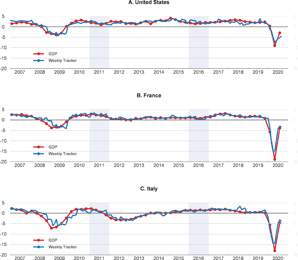
Note: The quarterly model is applied to 3-month moving averages of Google Trends series and yields monthly estimates that can be compared to quarterly GDP growth for February (Q1), May (Q2), August (Q3) and November (Q4). Shaded areas in 2011 and 2016 are years when the tracker is unavailable due to structural breaks in Google Trends data preventing the calculation of year-on-year growth rates in search intensities. Simulations are based on the latest GDP data, not the real-time vintages. For each quarter, the forecast is made five days after the end of the month, so 3-7 weeks before the GDP is published.
Source: Google Trends (https://www.google.com/trends); OECD Quarterly National Accounts; and OECD calculations.
Insights from the OECD Weekly Tracker
The COVID-19 crisis: A week-by-week analysis
The OECD Weekly Tracker provides early and timely indications about economic activity during the COVID‑19 crisis and the subsequent recovery (Figures 2.2 to 2.4) and is further validated by a close correlation with weekly movements in mobility (Woloszko, 2020). The magnitude of the shock to economic activity in March was extreme, as confirmed by GDP figures for the second quarter of 2020. The Tracker suggests that in a number of countries there was a rebound in April and May, with impetus slowing from June.
Figure 2.2. The OECD Weekly Tracker: United States
Weekly Tracker of GDP growth based on Google Trends
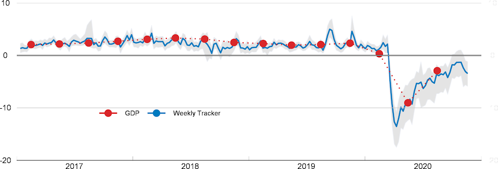
Note: The confidence band shows 95% confidence intervals.
Source: OECD Economic Outlook 108 database; and OECD Weekly Tracker.
The OECD Weekly Tracker suggests that this crisis caused major fluctuations in economic activity which were too abrupt to be captured by monthly indicators. Between 2017 and 2019, a high‑frequency proxy of GDP growth would not have added much useful information (Figure 2.2). However, in 2020, changes in economic activity were more rapid and pronounced, indicating a clear advantage of a weekly GDP proxy. During March 2020, the Weekly Tracker suggests that for the United States, year-on-year GDP growth fell from 2.4% during the first week to ‑10.2% in the last week, before reaching -14.7% in mid-April. In India, it fell from 1.6% in the second week to -15.3% in the last week of March, declines of a magnitude later corroborated by actual industrial production figures (‑16.3% year-on-year in April). The shock was also particularly sudden in many large European economies: for example, in the United Kingdom, the Weekly Tracker suggests that annual GDP growth fell from 0.4% to -20% in the course of March, reaching -24% in mid‑April. In contrast, in addition to being subject to longer publication delays, lower-frequency indicators provide a less detailed picture of both the pattern of the downturn and the recovery dynamics, when activity is changing rapidly.
Figure 2.3. The OECD Weekly Tracker: selected advanced G20 economies in 2020
Weekly Tracker of GDP growth based on Google Trends
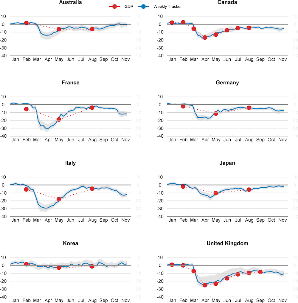
Note: The blue confidence band shows 95% confidence intervals. Red dots representing GDP growth are official outturns except for the third quarter of 2020 for Australia, which is the Economic Outlook estimate. Monthly GDP growth series are used when available (for the United Kingdom and Canada).
Source: OECD Economic Outlook 108 database; OECD Weekly Tracker; UK Office for National Statistics; and StatCan.
The OECD Weekly Tracker suggests that the immediate impact on GDP of the global pandemic was particularly heterogeneous across advanced economies (Figure 2.3). In France and Italy, where especially stringent lockdowns were implemented, activity is estimated to have fallen suddenly by around 29% below its 2019 level by early April (which is broadly consistent with GDP outturns for the second quarter). In countries where the lockdowns were less stringent, activity is estimated to have fallen slightly less abruptly: by 25% in the United Kingdom and by around 13-17% in Germany, Japan, Canada and Australia (again broadly consistent with GDP outturns for the second quarter). Korea, where epidemic control relied more on track-and-test than lockdown policies, had the lowest short-term drop, with the proxy measure of weekly GDP only falling by 4% below a year earlier in the worst week of April. While there is a clear impact from exiting lockdowns, the Weekly Tracker suggests the recovery in economic activity was much more gradual than following the initial impositions.
Figure 2.4. The OECD Weekly Tracker: emerging G20 economies in 2020
Weekly Tracker of GDP growth based on Google Trends
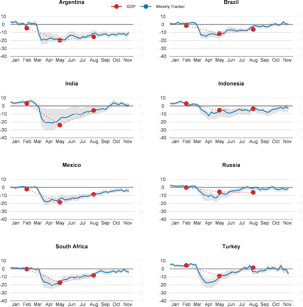
Note: The confidence band shows 95% confidence intervals. Red dots representing GDP growth are official statistics except for the third quarter of 2020 where they are either Economic Outlook projections or the outturns when the latter are available (for Indonesia and Mexico).
Source: OECD Economic Outlook 108 database; and OECD Weekly Tracker.
Many emerging-market economies exhibit a similar sudden fall in activity based on the Weekly Tracker, although the rebound differs widely across countries (Figure 2.4). The initial shock to activity is estimated to be particularly strong in India (-20%), Mexico (-19%), South Africa (-19%), Argentina (‑18%), Turkey (‑15%) and Brazil (-13%) with regards to the same weeks of 2019. Russia and Indonesia were hit less hard, as the Weekly Tracker suggests that activity at the trough was around 11% lower than in 2019. The fall in activity was particularly swift in Argentina and India, which implemented very stringent confinement policies.
Latest insights from the Weekly Tracker: A stalling recovery below 2019 levels
The OECD Weekly Tracker indicates that the rebound started to slow in June, with the most recent estimates implying that activity stagnated in the third quarter of 2020 well below 2019 levels for most countries (Figure 2.5, Panel A). The out-of-sample performance of the Weekly Tracker for the third quarter appears credible when compared to available GDP outturns for the quarter, given the very volatile environment. Across the 28 countries where GDP growth for the third quarter had been released at the time of finalising this note, the mean absolute error in predicting year-on-year GDP growth was around one percentage point with no evidence of systematic bias, compared with actual falls in GDP for the median country of nearly 5% and variation in quarter-on-quarter growth of between 2% and 18% across countries. On the basis of the Weekly Tracker, the rebound was particularly weak in Argentina, where activity in the third quarter is estimated to be around 15% lower than its 2019 level, as well as Mexico, the United Kingdom, Colombia and Spain, with activity estimated around 8-10% lower than 2019 levels.
The OECD Weekly Tracker up to the second week of November also provides some insight as to which countries have the strongest momentum in activity in the fourth quarter of 2020 (Figure 2.5, Panel B). The tracker suggests that many non-European G20 countries will have positive growth, at least over the first half of the quarter, reflecting some loosening of lockdown stringency, especially in Chile, Argentina, Brazil, India and South Africa, or maintenance of a low level of lockdown stringency. In some countries, including Chile, India, Brazil and Korea, this rebound is predicted to result in the level of GDP in mid-November being higher than a year earlier. In contrast, the Tracker suggests that quarterly growth will be negative in many European countries, where the stringency of lockdown measures has recently been tightened.
Figure 2.5. Most recent predictions of the OECD Weekly Tracker
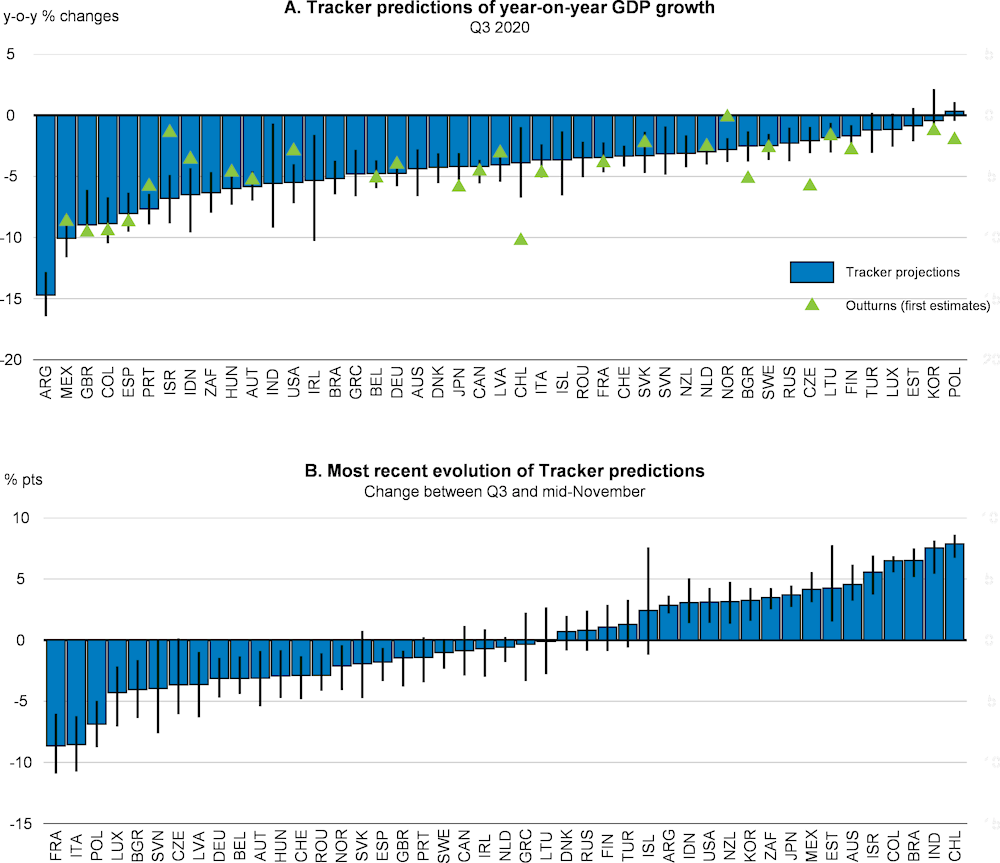
Note: In Panel A, the blue bars represent out-of-sample model projections of year-on-year GDP growth based on Google Trends and the black lines represent 95% confidence intervals around them. The triangles are GDP outturns for the third quarter. In panel B, the blue bars represent the difference between the average Tracker value over the first two weeks of November and the third quarter (Q3), while the black lines represent 95% confidence around them.
Source: OECD Economic Outlook 108 database; Google Trends (https://www.google.com/trends); and OECD Weekly Tracker.
Shifting consumption patterns
The Weekly Tracker model also provides insights into the main channels of weaker activity and at a more detailed level than national accounts. Figure 2.6 highlights the role of the fall of consumption of certain services in explaining the overall weakness in activity in France and Argentina, where the rebounds were particularly strong and weak respectively. In the second quarter of 2020, both countries experienced a strong shift in consumption patterns whereby search interest for interaction-based services (including events, performing arts, travel, hotels, sports and restaurants) decreased by around 30% while searches for food and drinks, household appliances and health-related issues increased by around 20%. Lower services consumption was only partially replaced by additional goods consumption resulting in lower overall spending, helping to explain negative model-estimates of year-on-year GDP growth. This pattern partly fades away in France in the third quarter, but not in Argentina, consistent with the different pace at which containment measures were relaxed. The potentially lasting effects of the virus circulation and mobility restrictions may thus explain part of the much weaker rebound in Argentina.
Figure 2.6. Google search intensities per spending categories
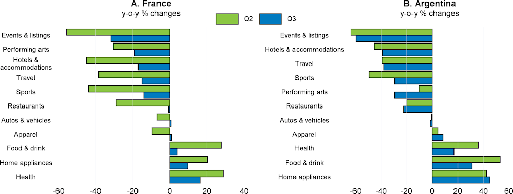
Note: Year-on-year growth rates in search intensities for selected search categories corresponding to spending categories (median over G20 and OECD countries).
Source: Google Trends (https://www.google.com/trends); and OECD calculations.
Bibliography
Abay, K., K. Tafere and A. Woldemichael (2020), “Winners and Losers from COVID-19: Global Evidence from Google Search”, World Bank Policy Research Working Paper, No. 9268, World Bank, Washngton D.C., https://papers.ssrn.com/abstract=3617347 (accessed on 1 September 2020).
Baker, S. R., N. Bloom and S. J. Davis (2016), “Measuring Economic Policy Uncertainty”, Quarterly Journal of Economics, 131(4), 1593-1636.
Bank of England (2020), How are we monitoring the economy during the Covid-19 pandemic?, https://www.bankofengland.co.uk/bank-overground/2020/how-are-we-monitoring-the-economy-during-the-covid-19-pandemic (accessed on 16 October 2020).
Benatti, N. et al. (2020), “High-frequency data developments in the euro area labour market”, ECB Economic Bulletin, 5/2020, https://www.ecb.europa.eu/pub/economic-bulletin/focus/2020/html/ecb.ebbox202005_06~a8d6c566d3.en.html (accessed on 16 October 2020).
Butler, D. (2013), When Google got flu wrong, http://dx.doi.org/10.1038/494155a.
Carrière-Swallow, Y. and F. Labbé (2010), Nowcasting With Google Trends in an Emerging Market, https://ideas.repec.org/p/chb/bcchwp/588.html.
Chen, S. et al. (2020), “Tracking the Economic Impact of COVID-19 and Mitigation Policies in Europe and the United States”, IMF Research, IMF.
Combes, S., and B. Clément (2016), “Nowcasting with Google Trends, the more is not always the better”, http://dx.doi.org/10.4995/CARMA2016.2016.4226.
Cournède, B., V. Ziemann and F. De Pace (2020), Housing amid Covid-19: Policy responses and challenges, OECD Policy Responses to Coronavirus (COVID-19), OECD, Paris.
Csáji, B. (2001), Approximation with Artificial Neural Networks, Faculty of Sciences, Etvs Lornd University, Hungary.
D’Amuri, F. et al. (2012), “The Predictive Power of Google Searches in Forecasting Unemployment”, Bank of Italy Temi di Discussione (Working Paper), No. 891.
Doerr, S. and L. Gambacorta (2020), “Identifying Regions at Risk with Google Trends: The Impact of Covid-19 on US Labour Markets”, BIS Bulletins, https://ideas.repec.org/p/bis/bisblt/8.html (accessed on 1 September 2020).
Ferrara, L. and A. Simoni (2019), “When Are Google Data Useful to Nowcast GDP? An Approach Via Pre-Selection and Shrinkage”, SSRN Electronic Journal, http://dx.doi.org/10.2139/ssrn.3370917.
Ginsberg, J. et al. (2009), “Detecting Influenza Epidemics Using Search Engine Query Data”, Nature, Vol. 457/7232, 1012-1014, http://dx.doi.org/10.1038/nature07634.
Gonzales, F., A. Jaax and A. Mourougane (2020), “Nowcasting aggregate services trade. A pilot approach to providing insights into monthly balance of payments data”, OECD, Paris.
INSEE (2020a), Les données « haute fréquence » sont surtout utiles à la prévision économique en période de crise brutale − Points de conjoncture 2020, Insee, Note de Conjoncture, https://www.insee.fr/fr/statistiques/4513034?sommaire=4473296 (accessed on 16 October 2020).
INSEE (2020b), Points de conjoncture 2020, Note de Conjoncture du 23 Avril 2020 , https://www.insee.fr/fr/statistiques/4481458.
Kliesen, K. (2020), “Tracking the U.S. Economy and Financial Markets During the COVID-19 Outbreak”, The FRED Blog, https://fredblog.stlouisfed.org/2020/03/tracking-the-u-s-economy-and-financial-markets-during-the-covid-19-outbreak/ (accessed on 16 October 2020).
Knotek, E. et al. (2020), “Consumers and COVID-19: A Real-Time Survey”, Economic Commentary (Federal Reserve Bank of Cleveland), 1-6, http://dx.doi.org/10.26509/frbc-ec-202008.
Morgavi, H. (2020), “A GARCH Model to Now-cast Private Consumption Using Google Trends Data”, forthcoming, OECD Economics Department Working Papers, forthcoming, OECD, Paris.
Narita, F. and R. Yin (2018), “In Search of Information: Use of Google Trends’ Data to Narrow Information Gaps for Low-income Developing Countries”, IMF Working Papers, No. 18/286, IMF, Washington DC.
OECD (2020a), OECD Economic Outlook, Interim Report September 2020, OECD Publishing, Paris, https://dx.doi.org/10.1787/34ffc900-en.
OECD (2020b), “Evaluating the Initial Impact of COVID-19 Containment Measures on Economic Activity”, OECD Policy Responses to Coronavirus (COVID-19), https://www.oecd.org/coronavirus/policy-responses/evaluating-the-initial-impact-of-covid-19-containment-measures-on-economic-activity-b1f6b68b/
OECD (2020c), “Issue Note 5: Flattening the unemployment curve? Policies to support workers’ income and promote a speedy labour market recovery”, OECD Economic Outlook, June, OECD Publishing, Paris, https://dx.doi.org/10.1787/1a9ce64a-en.
OECD (2020d), “Digital platforms and the COVID-19 crisis”, OECD Policy Responses to Coronavirus (COVID-19), OECD, Paris.
Varian, H. and H. Choi (2009), “Predicting the Present with Google Trends”, SSRN Electronic Journal, http://dx.doi.org/10.2139/ssrn.1659302.
Vermeulen, P. (2012), “Quantifying the Qualitative Responses of the Output Purchasing Managers Index in the US and the Euro Area”, ECB Working Paper, No. 1417, ECB, Frankfurt am Main, http://www.ecb.europa.euFax+496913446000http://www.ecb.europa.eu/pub/scientific/wps/date/html/index.en.html (accessed on 16 October 2020).
Woloszko, N. (2020), “A Weekly Tracker of activity based on machine learning and Google Trends”, OECD Economics Department Working Papers, No. 1634, OECD, Paris.